Steele Urges Coders to Abandon Accumulators for Automated Parallelism
Google TechTalks
Sequential loops and iterators bake in execution order that defeats multi-core chips, making associative divide-and-conquer abstractions essential for compilers to manage processors as automatically as garbage collectors handle memory.
Guy Steele argues that the core obstacle to automatic parallelization is not managing threads, but legacy sequential abstractions like accumulator loops and linear linked lists that force sequential dependencies. (0:25)
Using a trapped water histogram problem, Steele demonstrates four solutions: a classic sequential two-pass sweep, an associative divide-and-conquer merge using bitonic 'globs', a monoid-cached tree reduction, and an agnostic map-reduce formulation with parallel prefix/suffix scans. (8:34)
Associativity is identified as the fundamental algebraic prerequisite for parallel computing, allowing compilers and runtimes to dynamically schedule workloads across balanced binary trees rather than serial left-linear chains. (36:54)
Steele likens automated parallelism management to garbage collection, predicting that compiler-driven scheduling across heterogeneous hardware will eventually succeed manual threading to prevent codebases from needing rewrites every five years. (46:18)
Detailed notes
## Background
This Google Tech Talk was presented by Guy L. Steele Jr. on December 1, 2015, and published to YouTube by Google TechTalks on January 28, 2016. The presentation explores a deceptively simple geometrical problem—computing trapped rainwater on a histogram—to compare a classic sequential solution against three parallelizable approaches, examining their algorithmic tradeoffs, mathematical properties, and language abstractions.
## TL;DR
Steele argues that modern programmers should abandon sequential accumulator loops in favor of computational independence and associative divide-and-conquer abstractions. Using the trapped rainwater histogram puzzle as a running case study, he walks through four distinct implementations: a traditional two-pass sequential sweep, an associative 'bitonic globs' monoid reduction, a two-pass parallel traversal using monoid-cached trees, and a declarative MapReduce formulation built on parallel prefix scans. He demonstrates how higher-level algebraic expressions allow compilers to optimize representations and defer sequential versus parallel scheduling decisions. Ultimately, he posits that automated parallelism management represents the next essential evolution in programming portability, directly mirroring the historical adoption arc of automated garbage collection.
## Atmosphere & style
The presentation carries the warmth, dry wit, and intellectual rigor of an elder statesman of computer science speaking comfortably to a room of peers. Steele punctuates complex algebraic concepts and dense slide code with self-effacing humor, Monty Python references, and historical anecdotes spanning from Hollerith tabulating cards to Fortran compiler pioneers. The pacing moves smoothly from an energetic conceptual manifesto to granular data-structure walkthroughs, culminating in an engaging, interactive Q&A session that feels like an intimate masterclass on the future of language design.
## Bulletin
- [00:25](https://www.youtube.com/watch?v=ftcIcn8AmSY&t=25s) Guy Steele argues that the core obstacle to automatic parallelization is not managing threads, but legacy sequential abstractions like accumulator loops and linear linked lists that force sequential dependencies.
- [08:34](https://www.youtube.com/watch?v=ftcIcn8AmSY&t=514s) Using a trapped water histogram problem, Steele demonstrates four solutions: a classic sequential two-pass sweep, an associative divide-and-conquer merge using bitonic 'globs', a monoid-cached tree reduction, and an agnostic map-reduce formulation with parallel prefix/suffix scans.
- [36:54](https://www.youtube.com/watch?v=ftcIcn8AmSY&t=2214s) Associativity is identified as the fundamental algebraic prerequisite for parallel computing, allowing compilers and runtimes to dynamically schedule workloads across balanced binary trees rather than serial left-linear chains.
- [46:18](https://www.youtube.com/watch?v=ftcIcn8AmSY&t=2778s) Steele likens automated parallelism management to garbage collection, predicting that compiler-driven scheduling across heterogeneous hardware will eventually succeed manual threading to prevent codebases from needing rewrites every five years.
## Key takeaways
- [00:25](https://www.youtube.com/watch?v=ftcIcn8AmSY&t=25s) Programmers should design for computational independence rather than explicit concurrency coordination.
- [02:16](https://www.youtube.com/watch?v=ftcIcn8AmSY&t=136s) Traditional sequential accumulators create left-linear computation trees running in serial O(n) time, making automatic parallelization nearly impossible.
- [05:34](https://www.youtube.com/watch?v=ftcIcn8AmSY&t=334s) Linearly linked lists enforce sequential pointer chasing, whereas balanced three-case decomposition enables parallel evaluation with logarithmic depth.
- [08:34](https://www.youtube.com/watch?v=ftcIcn8AmSY&t=514s) The trapped water histogram problem requires computing individual water heights constrained by the minimum of the maximum barriers to the left and right.
- [10:09](https://www.youtube.com/watch?v=ftcIcn8AmSY&t=609s) The classic sequential approach requires a forward sweep for left maximums, a backward sweep for right maximums, and can be optimized into two passes via loop fusion.
- [13:31](https://www.youtube.com/watch?v=ftcIcn8AmSY&t=811s) A pure divide-and-conquer approach models histogram segments as bitonic 'globs' whose pairwise merging operator must be proven strictly associative.
- [23:35](https://www.youtube.com/watch?v=ftcIcn8AmSY&t=1415s) Monoid-cached trees persistently store subtree summaries at internal nodes, enabling parallel prefix scans with O(log n) span.
- [29:13](https://www.youtube.com/watch?v=ftcIcn8AmSY&t=1753s) Parallel prefix scans generalize everyday computations like checkbook ledgers into parallelizable tree sweeps.
- [33:27](https://www.youtube.com/watch?v=ftcIcn8AmSY&t=2007s) Abstracting the algorithm into map-reduce and prefix/suffix primitives decouples problem specification from execution strategy.
- [33:27](https://www.youtube.com/watch?v=ftcIcn8AmSY&t=2007s) Inlining abstract operations followed by loop fusion yields the optimal sequential code, while inlining on computation trees with deforestation reproduces the optimal parallel code.
- [35:39](https://www.youtube.com/watch?v=ftcIcn8AmSY&t=2139s) The historical dominance of accumulators stems from 19th-century tabulating machines and early CPUs optimizing for extreme memory conservation over execution time.
- [38:42](https://www.youtube.com/watch?v=ftcIcn8AmSY&t=2322s) Associativity allows grouping flexibility for parallelism, while other algebraic properties like commutativity and idempotence grant compilers scheduling and optimization latitude.
- [40:31](https://www.youtube.com/watch?v=ftcIcn8AmSY&t=2431s) Standard procedural constructs like Java iterators and C-style for loops hard-code sequential commitments that forfeit automatic parallelization.
- [43:47](https://www.youtube.com/watch?v=ftcIcn8AmSY&t=2627s) Practical parallel systems must adopt pragmatic engineering, such as wide branching factors and dropping to sequential flat arrays at leaf thresholds.
- [46:18](https://www.youtube.com/watch?v=ftcIcn8AmSY&t=2778s) Automating parallel processor scheduling is the logical successor to automated garbage collection and is essential for long-term program portability.
- [49:45](https://www.youtube.com/watch?v=ftcIcn8AmSY&t=2985s) The cultural friction against adopting parallel abstractions mirrors the early 1970s controversy surrounding the elimination of GOTO statements in favor of structured programming.
Matt introduces Guy Steele, noting that he is a familiar figure known for his work on programming language specifications like Common Lisp and Java, which employees at Google likely use every day. Honoring Steele’s request to keep the introduction brief, Matt promptly hands over the podium to audience applause. Steele remarks that it is good to be at Google and notes several familiar faces in the room, including some he had not anticipated seeing. While presenting on parallel programming to a Google audience might feel like “preaching to the choir,” Steele explains that he brings a distinct perspective, having delivered a version of this talk at other institutions, including Harvard University just the month prior.
Steele lays out his central philosophy: software developers should not have to spend mental energy explicitly coordinating parallelism. The difficulty lies in human cognition and the limitations of traditional programming abstractions.
> “And I think the issue is not so much thinking about parallelism as such, as just thinking about independence of computation.”
Current programming languages obscure whether operations are actually independent. In particular, Steele targets a common design pattern that he considers fundamentally flawed for concurrency:
> “And so, in a nutshell, my slogan, my over-simplified slogan, is accumulators are bad.”
Instead, developers must embrace divide-and-conquer paradigms and respect underlying mathematical structures:
> “Divide and conquer is good.”
> “And I think that making programmers aware of algebraic properties of their code, and communicating some of those properties to the compiler, may be worthwhile.”
[02:16](https://www.youtube.com/watch?v=ftcIcn8AmSY&t=136s) Summing an Array: The Pitfalls of Sequential Accumulation
To ground his thesis, Steele presents a simple example: summing an array $x$ containing 1,000,000 numbers. He shows a standard iterative snippet and asks if it can be parallelized, immediately joking that it doesn't matter because there is already a bug—the programmer forgot to initialize `SUM = 0`. Once corrected, the code remains fundamentally flawed because the iterative `DO` loop forces an inherently sequential evaluation order. Steele points out that compilers have to perform heroic feats to untangle this logic, noting that Frances “Fran” Allen was awarded the ACM A.M. Turing Award for devoting her career to developing compilers capable of undoing such sequential code and turning it into something a parallel machine can actually execute.
Steele contrasts this with mathematical notation and language design:
- Mathematical notation uses $\Sigma$ (capital sigma). It can be parameterized sequentially like a `DO` loop ($\sum_{i=1}^{1{,}000{,}000} x_i$) or written compactly over a set, declaring *what* to sum without prescribing *how*.
- Fortran 90 provides the `SUM` intrinsic function, which leaves the evaluation strategy open rather than forcing an early commitment to sequential iteration.
When looking at the computational structure of an accumulation loop, it forms a binary computation tree with an elongated left-linear spine: element $x_1$ is added to 0, then $x_2$ to that result, sequentially cascading down. Attempting to make this loop parallel simply by tagging it with an instruction like `DO PARALLEL` immediately introduces race conditions, where parallel threads read an old sum, compute their addition, and overwrite other threads' results, causing dropped values. Resolving the race condition by making the update atomic restores correctness, but destroys parallelism:
> “We can add things in any order, but we can't add things simultaneously.”
The truly desirable execution structure is a balanced tree where pairs of numbers are added simultaneously. This reduces execution depth from linear time ($O(n)$) to logarithmic time ($O(\log n)$), provided sufficient processor resources are available to exploit the tree's width.
```mermaid
flowchart TD
accTitle: Linear Accumulation Spine vs Balanced Tree Reduction
accDescr: Diagram contrasting an inherently sequential left-linear accumulator spine with a parallel balanced tree reduction.
[05:34](https://www.youtube.com/watch?v=ftcIcn8AmSY&t=334s) Data Decomposition: List Length in Lisp vs. Haskell
Data representation directly dictates whether parallel execution is possible. Steele demonstrates this using Lisp list traversal. A standard linearly linked list consists of chained cons cells connected by pointers. If the program only has a pointer to the head of the list, it cannot jump to the fourth block without traversing the first three:
> “And linearly-linked lists are, in fact, inherently sequential.”
The standard recursive formulation in Lisp checks if the list is empty (returning 0) or recurses on the rest of the list and adds 1 to the result. This approach has a total work of $\Theta(n)$ and a runtime delay of $\Omega(n)$ because pointer chasing is fundamentally serial.
Steele draws an analogy to Peano arithmetic, where the number 5 is encoded as $0 + 1 + 1 + 1 + 1 + 1$. While functional, it is far less efficient than binary positional notation:
- Standard right-to-left addition on binary numbers runs in time linear to the length of the representation, which is logarithmic in the magnitude of the number itself.
- Incorporating carry-lookahead logic yields an additional logarithmic speedup, enabling addition in $O(\log \log n)$ time relative to the value's size.
To obtain parallel efficiency on lists, programs require a multiway decomposition paradigm. Steele illustrates this using Haskell pattern matching over three distinct cases instead of the traditional two-case Lisp recursion:
1. **Empty list:** Length is 0.
2. **Singleton list:** Length is 1.
3. **Concatenation ($a ++ b$):** The length is the length of $a$ plus the length of $b$.
The Haskell definition leaves the exact splitting mechanism abstract. The total work remains $\Theta(n)$, but the delay drops to $\Omega(\log n)$, assuming constant-cost splits into approximately equal halves. If the splits are uneven or splitting overhead is nontrivial, the runtime delay degrades toward $O(n)$.
[08:34](https://www.youtube.com/watch?v=ftcIcn8AmSY&t=514s) The Bar Chart Trapped Water Problem
Steele transitions from basic summations to the central case study of the presentation: a toy programming problem with four distinct solutions. He credits Dan Nussbaum and Steve Heller with suggesting the problem, noting that it might also be familiar to audience members from Google job interviews.
The problem input consists of an array of non-negative integers. This array represents a bar chart, where each integer denotes the height of a vertical bar at that position. The goal of the algorithm is to calculate how much water would be trapped between these bars after a rainfall.
[09:00](https://www.youtube.com/watch?v=ftcIcn8AmSY&t=540s) The Histogram Problem and the Sequential Insight
The problem begins with a collection of unit-width vertical bars forming a histogram-like figure. When water is poured over the structure, it acts as an irregular container: “It's kind of a funny-shaped bowl.” The core challenge is to determine the exact volume of water the diagram can hold. Guy Steele notes that while audience members may recognize the classic puzzle, there are many distinct ways to tackle it. His talk focuses on four: one sequential and three parallel approaches. The central insight enabling computation is that the total water can be determined by figuring out the water residing on top of each individual bar in isolation and summing the results. This decomposition breaks the problem into independent pieces, opening up possibilities for parallelism.
```mermaid
flowchart TD
accTitle: Bar Water Containment
accDescr: Diagram showing how water on an individual bar is bounded by maximum heights to its left and right.
subgraph Bounds ["Containment Bounds"]
L["Max height to left"]
R["Max height to right"]
M["Water level = min(Left, Right)"]
L --> M
R --> M
end
subgraph Calculation ["Individual Bar Water"]
B["Bar height x_k"]
M --> D["Water = Water level - x_k"]
B --> D
end
```
To build up to the first sequential algorithm, Steele breaks down how much water any single bar—such as one of height 2—can support. The water level directly above any bar is strictly constrained by the tallest structure to its left and the tallest structure to its right that can trap it. The effective water surface height is the smaller of these two lateral maximums; subtracting the bar's own height from that surface height yields the volume of water trapped above that specific bar.
- The overall problem reduces to determining, for every position in the array, the maximum height to the left and the maximum height to the right.
- For a bar at index $k$ with height $x_k$, its trapped water is $\max(0, \min(\text{max\_left}_k, \text{max\_right}_k) - x_k)$.
[10:09](https://www.youtube.com/watch?v=ftcIcn8AmSY&t=609s) Two Sweeps, Minima, and Fortress Implementation
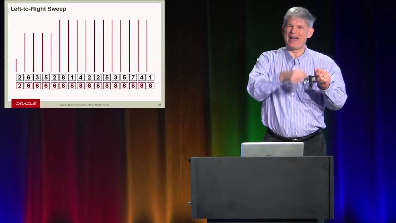
To compute these bounds sequentially across the entire array, the algorithm performs two directional passes using running accumulations. Steele jokingly introduces “the nasty word accumulation,” acknowledging that accumulators are inherently sequential. Starting from negative infinity, a left-to-right sweep maintains a running maximum, generating a non-decreasing profile of values across the bottom of the diagram (for example, stepping from 2 to 6, and eventually locking onto 8, the global peak). A complementary right-to-left sweep computes the maximums encountered from the opposite direction. Taking the pointwise minimum of these two sweeps yields the exact upper water boundary at every slot. Subtracting the original bar heights isolates each individual water column, and summing these columns yields the total volume, which evaluates to 35 for the 16-element example.
Steele then displays the sequential implementation and invites the audience to guess the programming language, quipping to specific attendees, “Anyone but Jan,” and “Anyone but David,” drawing laughter from the room before revealing it is Fortress. While Fortress is designed to resemble mathematical notation and looks like pseudocode, Steele assures the audience that it is fully operational: “But I assure you this is actually actual, functioning, running code, or at least it was as of three years ago, last time I checked it.” The routine, named `histogramWater`, operates on an array indexed by 32-bit integers (`ZZ32`) containing 32-bit integer values, immediately returning 0 for empty arrays to eliminate edge cases.
```mermaid
flowchart LR
accTitle: Three-Loop Sequential Execution Flow
accDescr: Pipeline of the three sequential loops computing left max, right max, and total water.
A["Left-to-Right Sweep<br/>(Max accumulation)"] --> B["Right-to-Left Sweep<br/>(Max accumulation)"]
B --> C["Pointwise Min & Subtract<br/>(Summation into total)"]
```
- **Loop Structure:** The straightforward implementation uses three separate loops: one for the left-to-right maximum accumulation, one for the right-to-left sweep, and a final loop that takes the minimum, subtracts the bar height, and accumulates the total sum.
- **Loop Fusion Optimization:** Compilers or programmers can optimize the sequential algorithm by fusing the final two passes: “And during the right-to-left pass, as we're accumulating the MAXs, then we can also do the rest of the accumulation as well.”
[13:31](https://www.youtube.com/watch?v=ftcIcn8AmSY&t=811s) Divide and Conquer: Bitonic Globs
Moving beyond sequential accumulation, Steele introduces a pure divide-and-conquer approach. Because the water above each bar can theoretically be handled independently, one might recursively decompose the input array down to individual bars, evaluate the water, and pairwise combine the results upward. A single bar contains no water, nor can a pair of bars contain any water. However, when pairs are merged into groups of four, water begins to collect; groups of four merge into groups of eight, and finally into the full array of 16 bars. Steele notes he deliberately picked an array of length 16 so the binary decomposition would divide evenly without corner cases.
```mermaid
flowchart TD
accTitle: Binary Decomposition Tree
accDescr: Hierarchical pairwise combination of bars from leaves to full 16-element glob.
subgraph Leaves ["Leaves (16 single bars)"]
B1["Bars 1..2<br/>(water = 0)"]
B2["Bars 3..4<br/>(water = 0)"]
B3["Bars 5..8"]
B4["Bars 9..16"]
end
subgraph Merges ["Pairwise Merging"]
G4["Groups of 4<br/>(begin trapping water)"]
G8["Groups of 8"]
G16["Final Combined Glob (16 bars)<br/>(total water = 35)"]
end
B1 --> G4
B2 --> G4
G4 --> G8
B3 --> G8
G8 --> G16
B4 --> G16
```
The key to an efficient merge step is recognizing that intermediate subproblems do not need their internal bar structures preserved. Steele refers to each intermediate subproblem as a “glob.” All that matters about a glob is the total volume of water it already contains and its external silhouette, which forms a bitonic outline. Steele explains that while monotonic means strictly increasing or decreasing, “Bitonic means it can go up and then it can go down—or, as they said of the Monty Python brontosaurus, it's very thin at one end, much, much thicker in the middle, and then very thin again at the far end, a-a-ahem.”
- **Combining Globs:** Merging two adjacent bitonic globs requires only their outlines and their current water totals (e.g., merging a left glob holding 11 units of water with a right glob holding 2 units).
- **Closure Property:** “The trick is to find an abstraction that can represent individual things. You can combine them, and the result is another instance of that same abstraction.”
- **New Water Computation:** When two globs are placed side by side, additional water is trapped in the depression between their peaks, producing a new combined bitonic outline whose total water is the sum of the left water, the right water, and the newly trapped intermediate water.
[16:23](https://www.youtube.com/watch?v=ftcIcn8AmSY&t=983s) Data Representation of Bitonic Outlines
To execute this merge in code, Steele formalizes the data structure representing a bitonic outline. Rather than tracking every bar coordinate, the outline is summarized as a series of horizontal plateaus characterized by their height and width. Instead of a naive list of height-width pairs, the representation explicitly isolates the global maximum plateau (the peak), because the combining algorithm relies heavily on comparing the peaks of adjacent globs.
```mermaid
flowchart LR
accTitle: Glob Data Structure Components
accDescr: The five fields that define a bitonic glob data structure.
subgraph Glob ["Bitonic Glob Data Structure"]
direction LR
L["Left plateaus<br/>(list of height, width)"]
P["Peak plateau<br/>(height, width)"]
R["Right plateaus<br/>(list of height, width)"]
W["Trapped water<br/>(integer)"]
end
L --- P
P --- R
R --- W
```
The resulting structure is a five-element tuple:
- A list of plateaus strictly to the left of the peak (monotonically non-decreasing in height).
- The height of the peak plateau.
- The width of the peak plateau.
- A list of plateaus strictly to the right of the peak (monotonically non-increasing in height).
- The total volume of water enclosed within the glob (a single integer).
Steele concludes by transitioning to the Fortress implementation of this abstraction, pointing out the top-level object declaration that encodes this five-element geometric summary.
[17:45](https://www.youtube.com/watch?v=ftcIcn8AmSY&t=1065s) The Glob Data Structure and Utility Routines
Guy Steele defines the internal architecture of a "glob." A glob is modeled as a record structure consisting of five specific components: the left outline list, the height of the top, the width of the top, the right outline list, and the total volume of trapped water contained within it. Operating over these records are several fundamental utility functions:
```mermaid
flowchart LR
accTitle: Glob Record Structure
accDescr: Diagram illustrating the five components that make up a bitonic glob record.
subgraph G["Glob Record"]
L["left outline"]
H["height of top"]
W["width of top"]
R["right outline"]
V["water volume"]
end
```
The first helper, `width`, takes a list $x$ of height-width pairs $(p, q)$ and sums all the widths ($q$ values). The second helper, `fill`, calculates how much water accumulates above an outline up to a proposed water level $m$. It processes each step in the list, extracts the bar's height $p$, subtracts $p$ from the proposed water height $m$, multiplies that difference by the bar's width $q$, and accumulates the total sum.
Steele then addresses the Fortress boilerplate code declaring the binary operator $\oplus$ (`O+`), which is used to perform large parallel reductions. In Fortress, declaring `object GlobReduction extends MonoidReduction[\Glob\]` serves a vital semantic purpose: “That's essentially a promise that the O+ operator, the combining operator, is going to be associative.” That mathematical promise of associativity justifies executing the reduction across a parallel tree. The declaration also provides an identity element (zero), though Steele bypasses those low-level mechanics to focus on the geometric algorithm.
[19:00](https://www.youtube.com/watch?v=ftcIcn8AmSY&t=1140s) Combining Bitonic Globs and Outline Splicing
Merging two adjacent bitonic globs requires handling three distinct geometric cases based on the relationship between their peaks:
1. The left peak is strictly higher than the right peak.
2. The right peak is strictly higher than the left peak.
3. Both peaks share the exact same height.
Each case fills in the intervening valley with water up to the lower peak's height, effectively expanding a plateau and bridging the two outlines into a single composite bitonic shape. Steele walks through the middle case in detail (viewed from the audience's perspective): the resulting outline on one side can directly reuse parts of the lower glob, but the opposite side must be assembled from three distinct segments: the lower glob's outline, a new bridge spanning the water, and a sliced portion of the higher glob's outline.
To extract that precise portion of the higher glob, a utility function splits a height-width list into three parts: the section strictly below a target height, the section strictly above it, and any flat segment sitting exactly at that height. Steele displays the full implementation of the binary $\oplus$ operator over globs. Acknowledging that “it's a bit of a mess,” he highlights the core invariant: it is a closed binary operation that accepts two globs and returns a new glob of the exact same type.
```mermaid
flowchart TD
accTitle: Combining Two Bitonic Globs
accDescr: Branching logic for the O+ binary operator depending on peak height comparison.
In["Compare Left Peak Height vs Right Peak Height"] --> L["Left Peak > Right Peak"]
In --> E["Left Peak == Right Peak"]
In --> R["Left Peak < Right Peak"]
L --> M["Fill valley & bridge outline"]
E --> M
R --> M
M --> Out["Single Combined Bitonic Glob"]
```
The sheer complexity of this operator raises a formal verification challenge: can we actually prove that $\oplus$ is associative? One could inline both expansions—$(a \oplus b) \oplus c$ and $a \oplus (b \oplus c)$—and apply symbolic source transformations by hand to confirm they reduce to identical normal forms. Steele remarks on having done this tedious exercise manually: “I've done that. It's a pain. It'd be nice to have a theorem prover do it, or a theorem prover built into a compiler—even better.” Because the Fortress source code explicitly promised a monoid, the compiler is informed of the intended associativity, making automated proof checking or property-based testing an ideal fit.
[21:47](https://www.youtube.com/watch?v=ftcIcn8AmSY&t=1307s) The Monoid Reduction One-Liner
With the $\oplus$ operator defined, Steele demonstrates the end-to-end reduction. Every individual element in the input array is converted into a singleton bitonic glob holding zero water:
> “So given singleton bitonic globs, we put water on top of them. There it is. None of them hold water. Maybe the whole argument doesn't hold water.”
Because $\oplus$ is associative, the evaluation order does not affect the final answer. The evaluation can be organized as a balanced binary reduction tree, allowing the runtime scheduler to execute it sequentially or in parallel depending on hardware efficiency. The reduction traverses the tree, combines all globs into a single master outline containing the trapped water volume (evaluating to 35 on the running example), and reaches in to project out the accumulated water component.
In Fortress, after all the supporting machinery is built, the final program collapses into a single line of code:
- Map every bar $v$ in array $x$ to a singleton glob.
- Reduce the collection using big $\sum$-style reduction with $\oplus$.
- Extract the water field from the final result.
Steele reflects on the trade-offs of this approach: “Well, it was very, very clever to be able to write this solution as a one-liner, once we built up this very complicated data structure and its associated operations.”
[23:35](https://www.youtube.com/watch?v=ftcIcn8AmSY&t=1415s) Introducing the Monoid-Cached Tree
Seeking a simpler, more systematic alternative to the complex glob algebra, Steele re-examines the original sequential algorithm's left-to-right sweep and introduces the concept of a **monoid-cached tree**. Rather than treating operations as ephemeral reductions, this approach constructs an explicit, persistent tree in memory where every internal node caches the monoid summary of all leaves in its subtree.
```mermaid
flowchart TD
accTitle: Monoid-Cached Tree Construction
accDescr: Bottom-up binary tree where internal nodes cache the pairwise maximum of child nodes.
subgraph Leaves["Leaf Layer (Array Elements)"]
L1["v1"]
L2["v2"]
L3["v3"]
L4["v4"]
end
subgraph Intermediate["Internal Node Layer"]
P1["max(v1, v2)"]
P2["max(v3, v4)"]
end
subgraph RootNode["Root Layer"]
R["max(subtree left, subtree right)"]
end
L1 --> P1
L2 --> P1
L3 --> P2
L4 --> P2
P1 --> R
P2 --> R
```
For this problem, the monoid operation is pairwise $\max$, whose identity element is $-\infty$. Steele shows the corresponding Fortress code defining the algebraic data type:
- A `trait CachedTree` comprising three object variants: `NullNode`, `SingletonNode`, and `PairNode`.
- An empty list produces a `NullNode` containing $-\infty$.
- A single-element list produces a `SingletonNode`.
- Larger lists are divided into roughly equal halves, which are recursively evaluated in parallel using Fortress tuple expressions (`(a, b)`):
> “Fortress allows the two expressions in a tuple expression to be computed independently. So there is a potential for parallelism there.”
The resulting subtrees are then stored in a `PairNode` alongside their cached maximum.
[25:50](https://www.youtube.com/watch?v=ftcIcn8AmSY&t=1550s) Two-Pass Up-Down Sweeps in Logarithmic Depth
Once the tree is built from bottom to top, a second, top-down parallel pass evaluates the prefix maximums. As execution descends from the root, information shifts horizontally across the structure:
```mermaid
flowchart TD
accTitle: Parallel Prefix Down-Sweep
accDescr: Downward propagation where cached values from left children pass to right children to compute prefix maximums.
Root["Root Node (Pass info across midpoint: Jump dist 8)"]
LChild["Left Child (Depth 1)"]
RChild["Right Child (Receives Left Summary)"]
Root --> LChild
Root -->|"cross-link left to right"| RChild
LChild --> LGrand1["Left Grandchild"]
LChild -->|"jump dist 4"| LGrand2["Right Grandchild"]
RChild --> RGrand1["Left Grandchild"]
RChild -->|"jump dist 4"| RGrand2["Right Grandchild"]
```
At the root level, the summary value of the entire left half jumps directly across a distance of 8 to inform the right half. At each successive layer downward, values are passed from each left child to its corresponding right sibling. Because the tree has logarithmic height, information propagates to every leaf in $O(\log n)$ parallel steps rather than the $O(n)$ steps required by a sequential scan.
Because the underlying $\max$-cached tree is entirely symmetric without any directional bias, the exact same tree can be reused to compute the suffix maximums (the right-to-left sweep) simply by reversing the direction of data exchange—passing values from right children to left children. Steele notes that an implementation can interleave both sweeps within the same recursive traversal: as each node is visited, it coordinates downward data transfers in both directions simultaneously, synthesizing the left-to-right and right-to-left arrays in a single unified pass.
[27:40](https://www.youtube.com/watch?v=ftcIcn8AmSY&t=1660s) The Monoid-Cached Tree Implementation
Guy Steele walks through the concrete Fortress implementation of the histogram water problem using a monoid-cached tree. Given an input list $x$, the top line of the code constructs its MAX-cached tree and feeds it directly into a recursive routine called `process`. This helper function executes the bidirectional (left-to-right and right-to-left) sweeps by passing down the running maximums and swapping information between children. Because the underlying data structure is a tree, the implementation cleanly mirrors its shape, dispatching across exactly three cases: `NullNode`, `SingletonNode`, and `PairNode`.
```mermaid
flowchart TD
accTitle: Monoid-Cached Tree Processing
accDescr: Processing a PairNode by recursively evaluating left and right subtrees in parallel via the plus operator.
subgraph TreeEval["Tree Traversal"]
P["PairNode"] --> L["process(left subtree)"]
P --> R["process(right subtree)"]
end
subgraph IndependentArgs["Fortress Independent Evaluation"]
L --> PLUS["Binary Operator (+)"]
R --> PLUS
end
PLUS --> S["Total Water"]
```
Parallelism emerges naturally in the `PairNode` method. When handling a pair node, the function calls `process` on the left subtree and `process` on the right subtree, joining the two results as arguments to the binary `+` operator. In Fortress, whenever a binary operator has two argument expressions, the language semantics allow the compiler to execute them independently if it chooses. Steele emphasizes the architectural economy of this approach compared to the earlier bitonic glob attempt:
- The implementation spans only two pages of code instead of four or five.
- It completely dispenses with the intricate "bitonic glob" representation and avoids inventing bespoke operators like $\mathcal{O}+$ or defining specialized `Big-O+` reductions.
- It introduces a reusable abstraction—the monoid-cached tree—that serves as a versatile foundation for standard library algorithms.
[29:13](https://www.youtube.com/watch?v=ftcIcn8AmSY&t=1753s) Parallel Prefix and the Checkbook Metaphor
Looking closely at the left-to-right sweep, Steele points out that the pattern “smells familiar” because it is fundamentally an instance of a parallel prefix operation. To explain parallel prefix to anyone unfamiliar with the formal concept, he turns to an everyday banking analogy:
> “Suppose you've got a checkbook—if you keep a checkbook. I keep a checkbook. A lot of people just use online statements and depend on the computer to do it. But if you keep a checkbook by hand, you know that you enter deposits and debits in the form of checks, and you keep a running balance. And at every step, the running balance is the result of adding to the previous running balance, either the deposit you made or subtracting the check you wrote.”
When represented as an array of positive and negative transactions, computing the running balances corresponds precisely to computing the prefix sums of the array. Formally, given an array of elements, a parallel prefix operation computes the reduction across every prefix: the first element, the sum of the first two, the sum of the first three, and so on.
Although usually computed left-to-right sequentially, prefix scans possess well-known, efficient parallel formulations. Steele notes that using a monoid-cached tree is one of several standard strategies documented in the computer science literature. Abstracting away the mechanics, Steele introduces concise mathematical notation for Fortress:
- A `MAX` operator with a rightward arrow overhead ($\overrightarrow{\mathrm{MAX}}$) designates a left-to-right parallel prefix sweep.
- A `MAX` operator with a leftward arrow overhead ($\overleftarrow{\mathrm{MAX}}$) designates a right-to-left sweep (a parallel suffix).
- Users do not need to specify the low-level implementation; the runtime and compiler decide whether to evaluate the operator sequentially or in parallel, identical to how a $\sum$ (big sigma) reduction is treated.
[31:23](https://www.youtube.com/watch?v=ftcIcn8AmSY&t=1883s) MapReduce in Mathematical Notation
With parallel prefix and parallel suffix abstracted into standard library operations, all boilerplate evaporates, yielding an executable, one-line Fortress expression built around a $\sum$ operator. The algorithm proceeds across three distinct phases:
```mermaid
flowchart LR
accTitle: One-Line MapReduce Histogram Solution
accDescr: Pipeline showing data generation via parallel prefix/suffix and zip, followed by element-wise mapping and summation.
subgraph Gen["Generate Phase"]
L["List x"]
P["Prefix MAX (x)"]
S["Suffix MAX (x)"]
L & P & S --> Z["zip(x, prefix, suffix)"]
end
subgraph MapRed["Map & Reduce"]
Z --> M["Map: min(left, right) - v"]
M --> SUM["Reduce: Summation (Big Sigma)"]
end
```
First, the generate step evaluates three lists: the original list $x$, its parallel prefix MAX, and its parallel suffix MAX. A compiler can choose to evaluate these concurrently across separate processors or fuse them into unified traversal loops. Next, Fortress's `zip` operator (adopted from Haskell) binds the three lists together, effectively transposing a 3-tuple of arrays into an array of 3-tuples: $(v, \textit{left}, \textit{right})$. In this tuple, $v$ represents the bar height, while $\textit{left}$ and $\textit{right}$ represent the maximum bounding heights computed by the prefix and suffix scans.
Second, the mapping phase computes the body expression of the big sigma for each tuple: $\min(\textit{left}, \textit{right}) - v$, representing the trapped water above that specific column. Finally, the reduction phase sums all individual water quantities using $\sum$.
Steele highlights this combination of generator, mapping body, and reduction operator as a quintessential MapReduce pipeline expressed in native mathematical syntax:
> “So this is map-reducing math notation. And I think this is actually a really good way to program, not only in the large, but also in the small, even for small stuff like this.”
[33:27](https://www.youtube.com/watch?v=ftcIcn8AmSY&t=2007s) The Core Argument: Decoupling Algorithms from Execution Strategy
Addressing whether this one-line implementation is sequential or parallel, Steele explains that the beauty of the code is that it refuses to commit to either. Prefix computation, suffix computation, and each instance of the inner mapping expression are completely independent. A compiler can inline the sequential definitions of `prefix`, `suffix`, and `zip`, producing nested for-loops, and then apply standard loop fusion to derive the optimal two-pass sequential solution. Steele confirms he has validated this manually: “And I don't have a compiler that does that automatically, but I have done that transformation by hand. This is about the biggest program I can do it by hand on.”
Conversely, if the compiler targets a parallel architecture, inlining parallel operator definitions produces operations over computation trees. Applying deforestation—which Steele characterizes as “loop fusion on trees”—transforms the exact same source code into the efficient two-pass parallel algorithm built on monoid-cached trees. Steele summarizes the central thesis of his presentation:
> “So this is the main point of the talk, is that it's possible to write solutions to problems that don't have a commitment as to whether to be sequential or parallel. And then downstream, either optimization at compile time, or decisions made at runtime, can make decisions about whether to be sequential or parallel.”
[35:39](https://www.youtube.com/watch?v=ftcIcn8AmSY&t=2139s) The History and Bias of the Accumulation Strategy
Steele steps back to analyze why programmers default so heavily to sequential architectures: the widespread addiction to the *accumulation strategy*. In accumulation, an algorithm starts with an empty base state and incrementally folds each input into the running total.
Because the incremental update step accepts an existing intermediate result and a single new datum to yield an updated state, the operator is fundamentally asymmetric. This asymmetry forces any conceptual computation tree into an entirely lopsided, left-linear or right-linear list, making the algorithm inherently sequential.
Steele contextualizes this by examining hardware history:
- Accumulation matches a single sequential processor perfectly, which is why early computing hardware was designed specifically around this paradigm.
- In early 20th-century Hollerith tabulating machines processing punched card data for the census, the internal counting units were literally known as "accumulators."
- Through the 1960s and early 1970s, CPU hardware registers were widely called accumulators before industry vernacular shifted to the generic term "registers."
- While accumulators inherently demand linear time, their lasting historical appeal was their ability to drastically conserve memory space.
[36:54](https://www.youtube.com/watch?v=ftcIcn8AmSY&t=2214s) Accumulation vs. Divide-and-Conquer: The Associative Merge
Guy Steele contrasts the traditional sequential accumulation paradigm with divide-and-conquer. In the accumulation model, a programmer reads an item from memory, folds it into a running state, keeps the overall footprint small, and avoids generating intermediate data structures by stashing state in local or global variables. By contrast, a divide-and-conquer strategy takes every raw input and constructs an explicit singleton solution from it, then repeatedly merges those solutions—typically pairwise—up a tree. This approach trades space for time: intermediate structures often end up allocated on the heap, and the pairwise merge operation ($\oplus$) is inherently more complex than a simple in-place update.
However, the payoff comes from the type signature of the merge operator. While an accumulation operator consumes a solution and a raw input to yield an updated solution `(Solution, Input) -> Solution`, an associative merge operator combines two peer solutions `(Solution, Solution) -> Solution`. As Steele emphasizes, “And its associativity is the key to parallelism.” Searching for an associative combining operator often yields deeper algorithmic insights into the structure of the problem itself. Steele reflects on his own experience with the geometric challenge discussed earlier in the lecture: he was unable to realize that a monoid-cached tree was the ultimate answer until he had first built an intermediate combining structure ("the glob combining thing") and realized he did not have to commit to building the entire solution in a single pass.
```mermaid
flowchart TD
accTitle: Accumulation versus Divide-and-Conquer Topologies
accDescr: Visual comparison contrasting sequential accumulation with tree-based associative merging.
- In sequential accumulation, data structures are minimized and updates are performed incrementally in local variables.
- In divide-and-conquer, inputs are elevated to singleton solutions, which can require logarithmic passes and heap allocation for intermediate nodes.
- Identifying an associative operator permits two-pass strategies: building partial subsolutions in trees during pass one, and completing the final solution in pass two.
---
[38:42](https://www.youtube.com/watch?v=ftcIcn8AmSY&t=2322s) The Pragmatic Meaning of Algebraic Properties
Steele acknowledges that audiences often tune out when speakers start throwing around formal abstract algebra terms: “And this is the point when I find that the eyes of my audience tend to glaze over when I mention this thing.” People might vaguely recall associativity and commutativity from elementary school "new math," but terms like idempotence draw total blanks. Yet, Steele argues that these formal mathematical concepts translate directly into practical, intuitive rules that every programmer relies upon:
- **Associativity** means grouping does not matter: “Associativity just means the way you group them doesn't matter, and that is the key to parallelism.”
- **Commutativity** means evaluation order does not matter: items can be swapped freely when summing or computing maximums without altering the outcome.
- **Idempotence** means duplicates do not matter: addition is not idempotent ($x + x \neq x$), but finding a maximum is ($\max(x, x) = x$), meaning duplicate records do not distort the result.
- **Identity** means a particular value does not matter: an identity element can be included or omitted without changing the computation.
- **Zero** (an absorbing element) means no other values matter: Steele jokes, “I'm the king, and I trump everybody else,” noting that if a single zero is present in a chain of a million multiplications, the entire product collapses to zero regardless of the rest.
These algebraic invariants are valuable because they provide compilers and runtimes with crucial implementation "wiggle room." When an operator is known to be associative, the execution engine is liberated to reshape data representations and dynamically schedule work sequentially or across parallel cores depending on runtime resource constraints.
---
[40:31](https://www.youtube.com/watch?v=ftcIcn8AmSY&t=2431s) Why DO Loops and Iterators Are "So 1950s"
Steele argues that modern computing is trapped in an archaic mid-twentieth-century mindset. Core procedural idioms were invented in the 1950s and perfected over decades solely for sequential execution: Fortran DO loops and Lisp linked lists are literally over fifty years old. Even modern constructs like Java iterators carry this sequential legacy forward:
> “The Java iterator data structure commits you, and its API, commits you to a sequential processing paradigm.”
The moment a programmer initializes an accumulator, the battle for parallel execution is lost before it begins. As Steele puts it: “As soon as you say, well, first let's set SUM to zero, you're already hosed—you're already hosed. And as soon as you say, process sub problems in order, you lose.” In the same vein, he remarks that “A for loop of a C or Java kind is probably the worst possible way to say map,” because compilers must expend tremendous effort attempting to analyze whether loop iterations possess hidden loop-carried dependencies.
Steele shares how unlearning these sequential habits transformed his personal coding mindset. Whenever he types a simple declaration like `int x = 0;`, he describes an internal chorus of competing voices—analogous to the personified emotional characters in Pixar's *Inside Out*:
- One voice asks whether `int` is truly the appropriate datatype.
- Another voice complains that `x` is a lazy, uninformative variable name.
- A third wonders if the literal should be an integer or a floating-point constant.
- A newly added "nerd critic" voice urgently demands: “Are you sure you want an accumulator? Maybe there's a better way to do this.”
Steele notes that parallel languages should not be designed by taking an entrenched sequential language and bolting parallel features onto its margins. His work on the Fortress programming language attempted to address this fundamentally. The parallel mindset requires abandoning linear decomposition entirely: top-down, one should never split problems into "first and rest," but rather into equal halves; bottom-up, one should never update a null solution incrementally, but rather map inputs to singletons and merge them.
---
[43:47](https://www.youtube.com/watch?v=ftcIcn8AmSY&t=2627s) Pragmatic Engineering and the Parallel to Garbage Collection
Steele steps back to moderate his stance, acknowledging that while his theoretical manifesto is intentionally extreme, real-world software requires pragmatic engineering trade-offs:
> “I have put forward a rather extreme manifesto. And I wanted to make sure I got that manifesto in your face. And I'm going to back off slightly. In practice, engineering needs to be done.”
At the leaves of a computation tree, where the vast majority of allocations reside, allocating individual singleton objects on the heap is prohibitively expensive; saving memory at the leaves can cut a program's overall footprint in half. Practical systems should adopt wider tree-branching factors rather than strict binary trees. Steele points to Clojure—a JVM-based Lisp dialect—which uses 32- or 64-ary trees for its persistent data structures, noting that while 64 might not be mathematically optimal, it is vastly better than 2 and vastly better than 10 million. Developers can also leverage self-balancing data structures such as red-black trees and finger trees.
```mermaid
flowchart TD
accTitle: Hybrid Parallel and Sequential Tree Processing
accDescr: Diagram showing parallel tree decomposition at high levels transitioning to flat sequential arrays at leaf thresholds.
Crucially, efficient systems should exploit parallelism high in the recursion tree, but drop down to fast sequential processing and flat arrays once subproblems drop below a certain size threshold. Languages like Fortress experimented with dynamically inspecting integer ranges or array chunks at runtime to decide whether to divide them recursively across threads or sweep through them sequentially.
Steele concludes this section by contrasting the current resistance against divide-and-conquer parallelism with the historical reception of automated garbage collection. Invented in the late 1950s for Lisp, garbage collection spent decades being actively feared and rejected by mainstream programmers who refused to relinquish explicit memory management. It took decades of optimization, complex parallelization work throughout the 1980s and 1990s, and the widespread adoption of Java before automated storage management finally became standard practice. Steele anticipates that declarative, independent parallel problem decomposition will follow a similar historical path.
[46:18](https://www.youtube.com/watch?v=ftcIcn8AmSY&t=2778s) Parallelism Management as the New Garbage Collection
Guy Steele concludes his talk by drawing a direct historical analogy between memory management and parallel computing. Decades ago, programmers worried incessantly about caches, memory layout, and the performance penalties of automated memory. Over time, the software community accepted garbage collection: although manual memory allocation can theoretically be fine-tuned to extract peak performance, “doing it by hand is so terribly hard.” Developers chose to sacrifice a small amount of performance to free themselves from manual tracking, and decades of engineering progressively mitigated those overheads without ever eliminating them entirely.
```mermaid
flowchart TD
accTitle: Analogy between Storage Management and Parallelism Management
accDescr: Diagram illustrating how memory allocation parallels code allocation across architectures.
subgraph Storage["Storage Management (Historical Evolution)"]
S1["Automatic Assignment of Storage"]
S2["Allocates Data to Heterogeneous Memory (Cache, RAM, SSD, Disk)"]
S3["Overheads Reduced Over Decades of Engineering"]
end
subgraph Parallelism["Parallelism Management (Future Vision)"]
P1["Automatic Assignment of Processors"]
P2["Allocates Code to Heterogeneous Processors"]
P3["Initial Overheads Mitigated by Future Compiler Engineering"]
end
Storage -.->|"Conceptual Equivalent"| Parallelism
```
Steele argues that modern computing faces the exact same transition with parallel execution: “I argue that the management of parallelism is very much like garbage collection. It's the automatic assignment of processors, rather than the automatic assignment of storage.” As hardware architectures diversify into heterogeneous mixes of CPUs, accelerators, and memory hierarchies, automatic scheduling is the only practical path to long-term portability:
- “I think this is our only hope for true program portability, and not to have to keep rewriting code every five years.”
- Programming languages must be actively designed to encourage independent, non-sequential thinking so runtime systems can schedule tasks across arbitrary processor topographies.
- Steele closes his prepared remarks with an open invitation to the audience to help build this future, followed by applause from the Google engineers.
[48:19](https://www.youtube.com/watch?v=ftcIcn8AmSY&t=2899s) Q&A: Retrofitting Existing Languages vs. Starting From Scratch
Opening the floor for questions, an audience member heads to the microphone to ask whether modern mainstream languages can adopt these parallel concepts, pointing out that entirely new programming languages face enormous barriers to adoption. Steele agrees that history demonstrates how difficult new languages are to popularize, but notes that functional programming concepts have steadily filtered into imperative languages for years.
Features like map and reduce in Java were directly inspired by Haskell after Sun and Oracle language architects monitored functional language developments across 10 to 15 years. However, retrofitting these idioms onto an imperative backbone creates an ongoing tension. Programmers still have access to legacy iterators, keeping them bound to a sequential mindset. Steele notes that retiring old features through language decay is often more politically feasible than driving wholesale migration to a clean-slate system:
- Steele candidly reflects on his own experience leading the design of Fortress: “I gave Fortress only, at most, a 20% chance of becoming big and making it. And surprise, surprise, it is in the 80%.”
- Despite Fortress not achieving mainstream commercial adoption, the Julia community has shown keen interest in its design ideas to guide Julia’s own language evolution.
- Steele warns that bolting declarative primitives onto imperative bases remains imperfect: “The question is, how do you get old things to drop off?”
[50:32](https://www.youtube.com/watch?v=ftcIcn8AmSY&t=3032s) Q&A: Mental Complexity and the Parallel Prefix Pattern
An engineer questions whether the concise parallel solution presented earlier in the lecture imposes too high a mental tax on developers, noting that it required nearly thirty minutes of explanation to convince a room of Google engineers that an associative operator on a custom five-component tuple was correct. Steele humorously rejects the premise that he formally proved anything: “First of all, you flatter me in trying to make me think that I've actually proved the correctness of this program to you. I don't believe I have.” Rather, he gave an informal intuition and backed it up with empirical tests.
Steele acknowledges that real-world state machines with dozens of fields cannot easily be collapsed into a single associative operator and should instead be partitioned. The steeper hurdle, however, is a lack of widespread education. To illustrate, Steele polls the room: while every single engineer raises their hand to confirm they know what a summation operator is, only roughly fifteen individuals in the entire audience have ever worked with parallel prefix scans. Once idioms like parallel prefix become standard parts of computer science training, explaining such solutions will require no extra effort than explaining a loop counter.
Steele draws a parallel to the bitter debates surrounding the structured programming movement of the early 1970s:
- When computer scientists first proposed banning arbitrary `goto` statements in favor of structured blocks (`if-then-else`, `while-do`), developers felt paralyzed, arguing that systems code and operating systems were impossible without jumps.
- Steele recalls attending the 1972 ACM National Conference debate as a young student, watching figures like Bill Wulf defend the BLISS compiler as proof that systems software could run cleanly without `goto`.
- Just as structured control flow eventually covered 90% of sequential needs once community consensus formed, Steele expects that a compact vocabulary of parallel building blocks will eventually govern 90% of parallel software.
[54:51](https://www.youtube.com/watch?v=ftcIcn8AmSY&t=3291s) Q&A: Grammars, Parsers, and Sequential Recursion
A final questioner asks about recursion patterns in formal languages, pointing out that foundational definitions like regular expressions and programming grammars are almost universally taught using asymmetric induction: start with a base element and recursively attach items sequentially to one side. The attendee asks how language designers can break away from that deeply ingrained habit.
Steele responds that grammar authors intentionally rely on rigid left recursion or right recursion for a purely practical reason: traditional parser generators (like Yacc or Bison) are built to output sequential parsers, and asymmetric rules match their internal state-machine mechanics. If toolchains instead targeted parallel parsing algorithms, grammars could be structured around balanced, divide-and-conquer decompositions rather than linear left-to-right cascades.
[55:27](https://www.youtube.com/watch?v=ftcIcn8AmSY&t=3327s) The Cost of Merging Bitonic Globs
Reflecting on his practical experience designing parallel parsers, Guy Steele points out that when targeting automated parallel execution, developers often have to rethink and rewrite their grammars and regular expressions from the ground up. An audience member then asks about the computational cost of merging two bitonic globs in the divide-and-conquer algorithm presented earlier. Steele flips back approximately fifty slides to walk through the implementation line by line to evaluate its exact complexity.
```mermaid
flowchart TD
accTitle: Bitonic Glob Merge Cost Breakdown
accDescr: Diagram showing the breakdown of operations and time complexity when merging two bitonic globs.
subgraph MergeOps["Bitonic Merge Operation"]
direction TB
A["Input: Left & Right Outlines"] --> B["Three-Way Split Operator<br/>(Binary decomposition of outline)"]
B --> C["Constant-Time Boundary Work<br/>(Local pointer & value updates)"]
end
subgraph Complexity["Complexity Analysis"]
direction TB
B --> D["Split Cost: O(log n)"]
C --> E["Remaining Work: O(1)"]
D & E --> F["Total Tree Combine Time: O(log² n)"]
end
```
Scanning the code, Steele notes that nearly all of the outline stitching logic takes constant time, with one crucial exception: the three-way split operator. To find where the water level meets the surface and separate the necessary outline segment, the implementation performs a binary decomposition of the outline list. Because this search requires logarithmic time relative to the outline half-length, the combine step cannot run in constant time. Consequently, the total combine time across the tree is not $O(\log n)$, but rather $O(\log^2 n)$. As Steele remarks: “And I couldn't figure out a way to make that log factor disappear.”
- Steele emphasizes: “All the rest of it is constant time. The problem is that three-way split.”
- The overall combining step runs in roughly $O(\log^2 n)$ rather than ideal logarithmic span, and Steele invites better algorithmic solutions to strip out that stubborn logarithmic penalty.
- An audience member interjects to thank Steele for all the foundational software, language design, and tooling he has delivered throughout his career, prompting warm applause from the room.
---
[57:15](https://www.youtube.com/watch?v=ftcIcn8AmSY&t=3435s) Language Adoption: Julia, Haskell, and Mainstream Giants
The Q&A shifts to how these algorithmic concepts translate into modern programming languages. When an audience member asks which existing languages show genuine promise for supporting these structured parallel paradigms, Steele highlights Julia, Haskell, and Clojure as the primary languages intentionally exploring associative, divide-and-conquer parallel approaches. He notes that while a language like Scala possesses the technical capability for such work, its community has not prioritized parallel algorithmic constructs along this specific dimension.
The questioner observes that Julia, Haskell, and Clojure remain somewhat niche, wondering whether an overwhelmingly popular language like Python—which already includes functional primitives like `map` and `reduce`—could become the primary vehicle for these ideas. Steele acknowledges that while Python has an enormous user base, parallel exploration accounts for only a minor fraction of its community. By contrast, smaller communities like Julia are actively pushing the frontier. Steele brings down the house with a self-deprecating nod to his own research language: “And they're all more popular than Fortress, you know? So help me, Obi-Wan, you're my only hope.” He explains that he tours diverse developer communities precisely to spark interest, hoping someone will take these parallel abstractions in unexpected directions.
---
[58:50](https://www.youtube.com/watch?v=ftcIcn8AmSY&t=3530s) The Evolution of Programmer Inertia and "Religion Wars"
An attendee revisits Steele’s comparison between modern parallelization and the structured programming revolution of the 1970s. Given that the global population of software engineers is exponentially larger now than it was forty years ago, the attendee asks whether sheer collective inertia will prevent a handful of computer scientists and academic papers from shifting industry-wide programming habits.
Steele acknowledges that scale naturally creates inertia, but argues that today's development culture is far less hostile to novel concepts than the community was in the mid-twentieth century. In the 1960s and 1970s, industry veterans who had been writing code since the dawn of electronic computing in 1945 resisted change fiercely, dogmatically insisting that Fortran or COBOL were more than sufficient. Despite that entrenchment, small groups still managed to reshape the paradigm. Today, Steele observes far less ideological dogmatism:
> “So yeah, I think there's more inertia, but I think there's less resistance today to new ideas.”
He adds that modern engineers are pragmatic and willing to adopt unfamiliar programming techniques whenever it is demonstrated that those techniques solve tangible problems. The heated, factional disputes of early computing have largely subsided, with Steele observing: “I'm seeing a lot less of the programming language, religion wars, let's say, which was a term of technical art back in the '70s.”
---
[01:00:24](https://www.youtube.com/watch?v=ftcIcn8AmSY&t=3624s) Real-World Systems and User Interface Parallelism
The final question tackles how divide-and-conquer parallel models apply to everyday domains like user-interface (UI) engineering. Steele acknowledges that direct interaction handling with an individual human user is fundamentally sequential: “And part of the problem is that our users tend to be sequential. If only we had parallel users, then things might be easier.”
```mermaid
flowchart LR
accTitle: Parallel Opportunities in UI and Page Rendering
accDescr: Flow demonstrating sequential user input contrasting with potentially parallel content presentation.
subgraph SequentialInput["User Input Path"]
direction TB
User["Sequential Human User"] --> Events["Sequential Event Queue"]
end
subgraph ParallelPresentation["Display & Rendering Pipeline"]
direction TB
Doc["Document / Web Page"] --> Text["Process Main Body"]
Doc --> Ads["Process Ad Units"]
Doc --> Media["Decode Media Elements"]
Text & Ads & Media --> Display["Screen Compositor"]
end
Events -.->|"Triggers update"| Doc
```
However, Steele distinguishes user input from the rendering and presentation pipeline, where immense parallelism could be unlocked. He argues that web standards like HTML could have enabled far more concurrency had they been architected with parallel composition in mind from the beginning. Instead, web browsers must perform complex acrobatics to determine whether disparate elements—such as third-party advertisements and primary article text—can be parsed and rendered independently without mutual layout interference.
Ultimately, Steele frames parallel execution as a pragmatic engineering trade-off: developers must weigh whether the latency gains of running two or more cores on an interface task outweigh the coordination overhead, or whether those CPU cycles are better allocated elsewhere in the system. With that parting insight, Steele concludes the lecture to hearty applause.
## Notable quotes
> [40:31](https://www.youtube.com/watch?v=ftcIcn8AmSY&t=2431s) A for loop of a C or Java kind is probably the worst possible way to say map. — Guy Steele
> [46:18](https://www.youtube.com/watch?v=ftcIcn8AmSY&t=2778s) I argue that the management of parallelism is very much like garbage collection. It's the automatic assignment of processors, rather than the automatic assignment of storage. — Guy Steele
> [38:42](https://www.youtube.com/watch?v=ftcIcn8AmSY&t=2322s) Associativity just means the way you group them doesn't matter, and that is the key to parallelism. — Guy Steele
> [00:25](https://www.youtube.com/watch?v=ftcIcn8AmSY&t=25s) I think the issue is not so much thinking about parallelism as such, as just thinking about independence of computation. — Guy Steele
> [40:31](https://www.youtube.com/watch?v=ftcIcn8AmSY&t=2431s) The Java iterator data structure commits you, and its API, commits you to a sequential processing paradigm. — Guy Steele
## Mentioned
Guy L. Steele Jr., Google, Frances Allen, ACM A.M. Turing Award, Fortress, Haskell, Java, Common Lisp, Clojure, Julia, Scala, Python, Fortran, Peano arithmetic, Herman Hollerith, Sun Microsystems, Oracle, Bill Wulf, BLISS, Monty Python, Dan Nussbaum, Steve Heller
## Video description
Google Tech Talk, 12/1/2015, Presented by Guy L. Steele Jr.
ABSTRACT: We present a small but interesting geometrical problem and then examine four different computational approaches to solving it: a "classic sequential solution" and three different approaches that are amenable to parallel implementation, comparing them to highlight various advantages and disadvantages, including total work required and minimum time to solution. All four solutions are illustrated both pictorially and with working code. We argue that certain approaches work better than others if exploitation of parallelism is to be automated. There will also be at least one joke.
Guy Steele Jr. argues that the greatest impediment to parallel programming is the ingrained habit of sequential accumulation, proposing instead that algorithms express computational independence through associative algebraic operators that compilers can map dynamically to sequential or parallel hardware.
The Flaw of Sequential Accumulation
Steele targets the traditional accumulation pattern, where an algorithm initializes an accumulator variable and iteratively folds elements into a running total. This approach, rooted in 1950s Fortran DO loops and historical hardware architectures that conserved memory via physical accumulator registers, forces a computation into a left-linear evaluation spine of O(n) depth. Even contemporary constructs like Java iterators enforce this linear constraint. Attempting to parallelize such patterns directly through compiler directives introduces race conditions, while making loop updates atomic merely restores sequential correctness without achieving parallel speedup.
Data structures similarly dictate execution topology. Steele contrasts Lisp's linear linked lists, which require Omega(n) runtime delay due to serial pointer chasing, with multiway data representations in languages like Haskell that decompose structures into balanced halves. Using balanced trees, operations like list length or array reduction drop from linear depth to logarithmic runtime delay (O(log n)), provided execution environments possess the width to process sibling nodes simultaneously.
Four Approaches to Trapped Water (8:34)
To demonstrate alternative execution strategies, Steele explores the trapped histogram water problem across four formulations. The baseline sequential algorithm performs two directional sweeps across an array: a left-to-right pass calculating prefix maximums and a right-to-left pass computing suffix maximums. Taking the pointwise minimum of both boundaries and subtracting the individual bar height determines the water column above each bar. Summed across an array of 16 bars, this yields 35 units of water. Compilers can optimize this sequential version by fusing the suffix calculation with the volume accumulation into two passes.
Steele contrasts this with two tree-based parallel solutions. First, a pure divide-and-conquer approach models subproblems as 'bitonic globs' using a five-element tuple representing outline plateaus and trapped water. These globs combine pairwise via an associative merge operator that bridges internal valleys; however, binary searches within its three-way outline split degrade its combine step to O(log² n) time. To simplify this algebra, Steele introduces a second approach: a monoid-cached tree that caches pairwise maximums in intermediate nodes during an upward pass, followed by bidirectional parallel sweeps downward in O(log n) steps.
Decoupling Specification from Hardware Strategy (31:23)
Steele notes that the bidirectional sweeps on a monoid-cached tree are concrete instances of parallel prefix and suffix operations. Using formal notation in the Fortress programming language, the trapped water problem reduces to a one-line pipeline: generating prefix and suffix MAX vectors, zipping them with the original array into tuples, mapping each element to its local water level, and reducing the result using a summation operator. Steele characterizes this as expressing MapReduce within mathematical syntax.
The central value of this formulation is that it declines to commit early to either sequential or parallel evaluation. A compiler targeting a single processor can inline the definitions of prefix, suffix, and zip into nested loops and apply standard loop fusion to recreate the optimal two-pass sequential code. When targeting concurrent architectures, the compiler can inline tree-based parallel prefix definitions and use deforestation—loop fusion across trees—to construct the parallel monoid-cached tree algorithm without modifying source code.
Algebraic Contracts and Engineering Realities
Steele explains that algebraic properties grant compilers implementation flexibility. Associativity permits arbitrary grouping, commutativity allows reordering, idempotence allows duplicate processing without distortion, and identity or absorbing elements enable short-circuiting. An associative merge operator requires a signature combining two peer solutions, (Solution, Solution) -> Solution, unlike asymmetric accumulation updates that take an intermediate state and raw input, (Solution, Input) -> Solution.
Addressing real-world deployment, Steele acknowledges that theoretical binary divide-and-conquer creates prohibitive memory overhead if singletons are allocated on the heap for every leaf. Practical architectures must adopt hybrid approaches: dividing work across trees with wide branching factors (such as the 32- or 64-ary persistent trees used in Clojure) at upper levels, then dropping down to flat sequential arrays once subproblems fall below a size threshold.
Steele compares the future of parallel programming to the historical adoption of garbage collection, arguing that automatic processor scheduling will eventually replace manual thread coordination despite early performance compromises. However, questions remain regarding how quickly the broader industry can overcome educational deficits around concepts like parallel prefix and retrofit legacy imperative codebases.
## Background
本内容由 Google TechTalks 频道于 2016 年 1 月 28 日在 YouTube 平台发布,记录了 Guy L. Steele Jr. 于 2015 年 12 月 1 日在 Google 发表的现场技术演讲。页面简介指出,演讲围绕一个看似微小却极具启发性的几何蓄水问题展开,对比经典串行解法与三种支持并行实现的方案,探讨自动化并行挖掘与算法设计权衡,并穿插趣味典故。
## TL;DR
Guy Steele 提出了编写并行程序的精辟理念:优秀的并行编程往往要求程序员克制对底层的直接并发控制,转而专注发掘计算本身的“独立性”与代数结合律。他以经典且直观的“柱状图雨水收集”几何问题为切入点,层层拆解了四种计算形态——从依赖双向扫描的经典串行循环,到基于双调轮廓(Bitonic Glob)的纯分治树状规约,再到构建 MAX 缓存树(Monoid-cached Tree)与单次信息交换遍历,最终升华至基于并行前缀/后缀操作与 Map-Reduce 范式的优雅一行式表达。Steele 借此批判了 1950 年代遗留下来的单核累加器思维定势,主张通过赋予编译器解耦并行与顺序调度的自由,推动程序自动化并行走向如垃圾回收(GC)般的成熟工业标准。
## Atmosphere & style
整场讲座洋溢着计算机科学泰斗深入浅出的幽默感与举重若轻的大师风范,既有严谨的代数推演,又穿插着对 Fortress、Python 及巨蟒剧团台词的自嘲与调侃,现场掌声与笑声不断。面对满堂 Google 顶尖工程师,Steele 娓娓道来,从宏大的 40 年计算史跨度将当下的并行困局与 1970 年代结构化编程革命深度类比。问答环节则真实而尖锐,讲者不避讳复杂度和生态落地的现实难题,营造出一种兼具理论美感与深刻工程反思的高密度技术思辨氛围。
## Bulletin
- [00:25](https://www.youtube.com/watch?v=ftcIcn8AmSY&t=25s) Guy Steele 提出并行编程的核心原则在于“关注独立性而非刻意设计并行”,并直言“累加器是坏的,分治法是好的”,呼吁业界摆脱自 1950 年代延续至今的串行累加思维。
- [31:23](https://www.youtube.com/watch?v=ftcIcn8AmSY&t=1883s) 通过对直方图蓄水问题的四种解法对比,Steele 展示了借助并行前缀(Parallel Prefix)与并行后缀,可将原本多页的复杂逻辑浓缩为一行对顺序与并行保持中立的 Map-Reduce 风格数学表达式。
- [46:18](https://www.youtube.com/watch?v=ftcIcn8AmSY&t=2778s) Steele 将未来的并行管理演进类比为垃圾回收(GC)的历史:从早期的手工内存管理与开销担忧,逐步发展为将“代码到处理器的配置”全权委托给运行时系统的自动化并行。
- [55:27](https://www.youtube.com/watch?v=ftcIcn8AmSY&t=3327s) 尽管双调块(Bitonic Glob)分治方案具备严格的数学闭包与结合律,但其底层的三路切分算子引入了二分分解,导致整体时间跨度达到 O(log² n) 的复杂度瓶颈。
## Key takeaways
- [00:25](https://www.youtube.com/watch?v=ftcIcn8AmSY&t=25s) 并行编程的最佳实践是让程序员专注表达计算的相互独立性,将并行与顺序的具体调度决策交由编译器和运行时系统裁决。
- [02:16](https://www.youtube.com/watch?v=ftcIcn8AmSY&t=136s) 传统 DO 循环与累加器在语义上是固有串行的,二叉计算树呈现为深度为 O(n) 的线性脊柱,而平衡树归约则可将延迟压至 O(log n)。
- [05:34](https://www.youtube.com/watch?v=ftcIcn8AmSY&t=334s) 数据结构本身会决定代码的执行特征,线性单向链表在本质上是串行结构,无法直接推导并行,而支持均衡切分的数据结构才能释放并发潜能。
- [09:00](https://www.youtube.com/watch?v=ftcIcn8AmSY&t=540s) 直方图蓄水问题的经典串行解法通过从左至右与从右至左两趟扫描维护极值,取两者较小值减去单柱高度后再进行累加求和。
- [13:34](https://www.youtube.com/watch?v=ftcIcn8AmSY&t=814s) 纯分治方案将几何外廓抽象为包含峰值与两侧阶梯的“双调块(Bitonic Glob)”,实现了在两两合并时仅保留水量标量与外边缘的代数封闭性。
- [19:01](https://www.youtube.com/watch?v=ftcIcn8AmSY&t=1141s) 双调块合并代码包含三路切分以支持积水跨接,向编译器声明结合律承诺即可支持树状规约,但手动验证或证明结合律极其繁琐。
- [23:35](https://www.youtube.com/watch?v=ftcIcn8AmSY&t=1415s) Monoid 缓存树(MAX-cached Tree)通过自底向上建树并在自顶向下过程中完成子节点数据交换,能在单次遍历中同时得出双向扫描结果。
- [31:23](https://www.youtube.com/watch?v=ftcIcn8AmSY&t=1883s) 借助并行前缀与并行后缀运算,直方图蓄水问题可在 Fortress 中浓缩为一行 Map-Reduce 风格表达式,对底层执行是串行还是并行完全保持中立。
- [33:27](https://www.youtube.com/watch?v=ftcIcn8AmSY&t=2007s) 保持中立的高阶表达式允许编译器自由施展优化:内联串行定义即可通过循环融合退化为串行两趟扫描,内联并行定义则可通过去森林化转为树状并行。
- [35:39](https://www.youtube.com/watch?v=ftcIcn8AmSY&t=2139s) 累加范式(Accumulator)因契合单核架构与节省内存而统治了数十年,但其非对称的类型签名导致其无法满足结合律,彻底封死了并行可能。
- [38:42](https://www.youtube.com/watch?v=ftcIcn8AmSY&t=2322s) 结合律意味着分组无关性,是实现树状拆分并行调度的数学基石;而交换律、幂等性与零元等性质也为编译器提供了宝贵的优化活动空间。
- [43:47](https://www.youtube.com/watch?v=ftcIcn8AmSY&t=2627s) 工程落地中无需追求纯粹的细粒度并行,可采用增大树分支因子(如 Clojure 的 64 叉树)并在叶节点设置阈值回退至连续数组串行处理以优化开销。
- [46:18](https://www.youtube.com/watch?v=ftcIcn8AmSY&t=2778s) 代码到处理器的自动配置与分配就如同垃圾回收对内存的管理,初期的高开销必将随着软硬件技术的演进而被逐步消化,最终实现跨架构的程序可移植性。
- [50:25](https://www.youtube.com/watch?v=ftcIcn8AmSY&t=3025s) 当前开发者对并行前缀等概念的不适应,类似于 1970 年代推行结构化编程、废除 goto 时遭遇的阻力;当基础教育与核心原语普及后,心智负担将大幅下降。
- [55:27](https://www.youtube.com/watch?v=ftcIcn8AmSY&t=3327s) 双调块合并算法中由于三路切分算子需要对轮廓进行二分分解(O(log n)),导致并行树的整体计算跨度上升为 O(log² n) 的性能瓶颈。
- [01:00:24](https://www.youtube.com/watch?v=ftcIcn8AmSY&t=3624s) UI 交互中针对单用户的输入事件流具有强顺序性,并行收益有限;但内容呈现与 DOM 布局排版在良好解耦的架构下蕴含着巨大的并发潜力。
## Detailed walkthrough
### [00:25](https://www.youtube.com/watch?v=ftcIcn8AmSY&t=25s) 讲者介绍与并行编程的核心观点
主持人 Matt 向在座的 Google 工程师们介绍了 Guy Steele,指出大家可能对这个名字相当熟悉,因为他深度参与了多种主流编程语言规范的制定,其中就包括 Common Lisp 和 Java。Matt 笑称在 Google 办公室里肯定有人在用这些语言,并遵从 Guy Steele 的嘱咐,简短介绍后便将舞台交由他。
Guy Steele 登台后感谢了 Matt,看到台下有不少熟面孔(甚至包括一些意料之外的朋友)。他指出本次分享的主题是并行编程(parallel programming)。虽然在 Google 谈并行编程有点像“向唱诗班布道”(preaching to the choir),但他希望带来自己独特的视角,并将此前在哈佛等大学分享的理念传递给 Google。
Guy Steele 明确提出了他的核心论点:编写并行应用程序的最佳方式,是尽可能不去思考并行本身。人类大脑天生不擅长处理并行逻辑,因此系统需要关注点分离(separation of concerns)。比起刻意琢磨并行,程序员更应该思考计算的“独立性”(independence of computation)。然而,现代编程语言并没有提供足够的机制来帮助开发者表达或指出哪些计算是彼此相对独立的。他特别指出了自己的一个眼中钉(bugaboo)——累加范式(accumulation paradigm),因为累加在本质上往往是串行的。Guy Steele 直截了当地给出了自己的精辟总结:“我的过度简化版口号是:累加器是坏的,分治法是好的(accumulators are bad; divide and conquer is good)。”尽管分治是老生常谈的道理,但现代软件工程需要更严肃地对待它。此外,结合自身在应用代数领域的背景,Guy Steele 强调代数性质(algebraic properties)至关重要;让程序员意识到代码背后的代数性质,并把这些性质传达给编译器,会带来巨大的价值。
### [02:16](https://www.youtube.com/watch?v=ftcIcn8AmSY&t=136s) 数组求和的陷阱:串行循环、数据竞争与树状归约
为了具象化累加器的问题,Guy Steele 提出了一个简单的场景:假设有一个长度为 100 万的数组 `x`,我们需要计算其中所有元素的总和。他展示了一段基础循环代码,并反问台下:“这段代码可以并行化吗?”接着他幽默地自嘲道:“谁在乎呢,这段代码里有个 bug——我忘了初始化 `SUM`!”引发现场笑声。在更正了初始化为 0 之后,他进一步剖析:这段使用 `DO` 循环的代码本质上是糟糕的,因为它的语义是固有串行的(inherently sequential),聪明的编译器必须花费极大力气去“撤销”(undo)这种串行约束。Fran Allen 正是凭借一生致力于编写能够解开这类代码、将其重构成可供并行计算机运行代码的编译器,从而获得了图灵奖(Turing Award)。
相比之下,数学家在表达求和时使用大 $\Sigma$ 记号,或者像 Fortran 90 中的内建函数 `SUM` 那样,只声明“要做什么”(求一组数的和),而没有指定“怎么做”。Guy Steele 强调,核心就在于不要过早将计算策略定死。
```mermaid
flowchart TD
accTitle: Summation Computation Trees Comparison
accDescr: Sequential linear spine vs parallel balanced binary tree for summation
subgraph SEQ["串行累加树 (线性脊柱: 深度 O(n))"]
direction TB
S0["0 + x[1]"] --> S1["... + x[2]"]
S1 --> S2["... + x[3]"]
S2 --> SN["... + x[n]"]
end
subgraph PAR["分治并行树 (平衡二叉树: 深度 O(log n))"]
direction TB
P1["x[1] + x[2]"]
P2["x[3] + x[4]"]
P3["x[n-1] + x[n]"]
P12["Sum(1..4)"]
P1 --> P12
P2 --> P12
PALL["总和 SUM"]
P12 --> PALL
P3 --> PALL
end
```
在详细解析求和计算模型时,Guy Steele 探讨了三种执行方式与计算树形态:
1. **纯串行 DO 循环**:在二叉计算树中形成一条漫长的“线性脊柱”(linear spine)。开发者必须从 0 开始,依次加上 $x_1$、$x_2$ 直至最后,任何上层的加法都必须等待底层的加法完成,时间延迟为 $O(n)$。
2. **粗暴标记并行(Parallel DO)**:如果直接并发执行循环体,会产生致命的数据竞争(race condition)。多个线程同时读取 `SUM`、加上本地的 $x_i$ 并写回,相互覆盖,导致大量求和结果丢失。
3. **加原子锁(Atomic DO)**:若将读取、累加、写回封装为原子操作,虽然程序恢复了正确性且允许乱序相加,但仍然无法做到真正的“同时计算”(simultaneously),计算依然是串行阻塞的,根本没有带来吞吐量提升。
4. **两两归约的平衡计算树**:Guy Steele 指出:“我们真正期望的是将这 100 万个元素两两成对相加,得到的计算树高度与元素数量的对数(logarithm)成正比,而不是与元素数量本身成正比。”只要有足够的处理器硬件资源,算法就能在对数时间(log time)内完成计算。
### [05:34](https://www.youtube.com/watch?v=ftcIcn8AmSY&t=334s) 数据结构对并行的决定作用:从 Lisp 链表到 Haskell 分治
为了进一步阐明数据表示如何限制并发,Guy Steele 引入了他钟爱的 Lisp 语言,讨论如何计算链表的长度(length of a list)。在典型的 Lisp 链表中,数据由指针串联的节点组成。若只有一个指向表头的指针,程序员就必须顺着指针一步步向后寻址,根本无法在不遍历前驱节点的情况下直接访问第四个节点。
Lisp 的经典递归实现非常直观:若链表为空则返回 0;否则对除表头外的剩余链表(rest)递归求长度,并在此基础上加 1。这种方式的总计算工作量(work)是 $\Theta(n)$,但其延迟(delay)下界是 $\Omega(n)$。Guy Steele 指出:“数据可以决定代码的运行方式;线性链表在本质上是固有的串行结构(data can dictate the way code works. And linearly-linked lists are, in fact, inherently sequential)。”这正如皮亚诺算术(Peano arithmetic)用 $0 + 1 + 1 + 1 + 1 + 1$ 来表示数字 5,虽然可行,但采用二进制表示法效率要高得多——在进位传递加法器等结构支持下,二进制加法甚至能达到双重对数时间 $\log(\log n)$ 的极速。
随后,Guy Steele 对比了 Haskell 中的列表长度计算模型。通过三路分解(three-way decomposition),Haskell 可以将模式匹配扩展为:
- 空列表:长度为 0
- 单元素列表(singleton):长度为 1
- 多元素列表:将列表拆分为子列表 $a$ 与 $b$($a$ 与 $b$ 的连接构成原列表),分别递归求长度后再相加
该算法将求长问题转化为了多个 1 的求和问题。总工作量依旧是 $\Theta(n)$,但其时间延迟取决于切分列表的方式:如果每次都能以常数代价将列表切分成规模相近的两半,延迟就能优化至 $\Omega(\log n)$;如果切分极不均衡或者切分操作本身代价过高,性能就会退化到 $O(n)$ 甚至更糟。
### [08:34](https://www.youtube.com/watch?v=ftcIcn8AmSY&t=514s) 核心问题引入:条形图雨水收集/最大矩形问题
铺垫完上述理论背景后,Guy Steele 揭晓了本场演讲的核心玩具问题(toy programming problem)。他特别感谢了 Dan Nussbaum 和 Steve Heller 提供这道题目,并调侃这道题可能曾经出现在 Google 招聘的技术面试题库中。
该问题以一个整数数组为输入,数组中的每个整数均代表柱状图(bar chart)中对应柱子的高度。通过这个直观的几何学小问题,他将在后续内容中展示四种截然不同的计算方案:一种经典的串行解法,以及三种各具特色的并行实现,以此全面比较它们在总计算工作量与最小执行时间等维度的权衡。
### [09:00](https://www.youtube.com/watch?v=ftcIcn8AmSY&t=540s) 柱状图接水问题与经典串行解法
Guy Steele 首先明确了问题的物理模型:给定一组单位宽度的柱子排成一排,在上方倾倒水,整个结构如同一只形状奇特的碗。核心问题在于:这个图表总共能装下多少水?听众中不少人点头示意认出了这一经典题目。Steele 表示该问题有许多种解法,今天他将展示其中的四种——一种是经典的串行算法,另外三种则是适用于并行计算的方法。
要切入这个问题,最关键的直觉在于:“我们也许能够分别计算出每根柱子上方所容纳的水量,然后把它们全部加起来。”这种拆分将问题分解成了完全独立的局部片段,从而为潜在的并行化提供了可能。但在探讨并行之前,首先考察经典的串行实现。对于任何一根特定高度的柱子(例如图中一根高度为 2 的柱子),其上方能够容纳的水位高度,完全取决于其左侧最高柱子与右侧最高柱子中较矮的那一个($\min(\text{leftMax}, \text{rightMax})$)。用该水位上限减去柱子本身的高度,就得出了该位置上方实际蓄积的水量。
```mermaid
flowchart TD
accTitle: 串行算法的三阶段流程
accDescr: 展示从左至右扫描、从右至左扫描,以及逐柱计算水深并累加求和的全过程。
subgraph SweepStage["扫描计算边界"]
direction LR
L["从左至右扫描<br/>MAX 累积 (Left Max)"]
R["从右至左扫描<br/>MAX 累积 (Right Max)"]
end
subgraph ComputeStage["逐柱计算并求和"]
direction TB
M["取较小值:<br/>H = min(Left Max, Right Max)"]
W["计算单柱储水:<br/>Water = H - Bar Height"]
S["全数组求和:<br/>∑ Water = 35"]
end
SweepStage --> M
M --> W
W --> S
```
为了得到全数组每个位置的边界信息,算法按以下步骤执行:
1. **从左向右扫描**:初始值设为负无穷($-\infty$),沿数组从左向右推进并维护最大值累积(MAX accumulation)。以示例数据为例,遇到高度为 2 的柱子后累积值为 2,遇到高度为 6 的柱子后变为 6 并维持一段时间,直到扫到全局最高的 8 为止,之后均为 8。
2. **从右向左扫描**:以对称方式从右端向左执行最大值扫描,获取各位置右侧的最大高度。
3. **逐位取交集并作差**:在每个位置取左右最高柱子的最小值(图中以绿色短横线标出),随后减去该位置柱子本身的高度,即可精确得到各位置的水柱高度。
4. **求和得出结果**:对所有单柱上方水量执行大 $\Sigma$ 累加,在示例由 16 根柱子构成的数组中,计算得出的总蓄水量为 35。
---
### [11:15](https://www.youtube.com/watch?v=ftcIcn8AmSY&t=675s) Fortress 语言与串行代码优化
随后,Steele 在大屏幕上展示了该串行算法的实现代码,并向现场听众发问,看是否有人能认出这门编程语言。在观众低语后,他打趣道:“除了扬(Yahn),谁都可以猜。”引来全场哄堂大笑;接着他又笑着补了一句“除了大卫(David)”,因为他们参与过开发,看一眼便心知肚明。Steele 揭晓答案:这是 Fortress 语言。
> “这看起来可能很像伪代码——那是因为 Fortress 是一门专门设计成接近数学伪代码风格、并使用数学符号的编程语言;但我向大家保证,这确实是货真价实、能够实际运行的代码,或者至少三年前我最后一次测试它时它还是能跑的。” —— Guy L. Steele Jr.
```fortress
histogramWater(x: Array1[ZZ32, ZZ32]): ZZ32 = do
n = |x|
if n = 0 then 0
else
...
```
在这段名为 `histogramWater` 的程序中,输入参数是一个一维数组 `x`,数组索引与元素均采用 32 位整数(类型记为 `ZZ32`),函数最终返回一个 32 位整数蓄水量。代码开篇获取数组长度 $n$,并在 $n=0$ 时直接返回 0,干净利落地排除了边界退化情形。代码主体包含三个明确的循环遍历:
- 第一个循环执行从左向右扫描,将最大高度累积到 `left` 数组中;
- 第二个循环执行从右向左扫描,将最大高度累积到 `right` 数组中;
- 第三个循环遍历所有柱子 $k$,计算 $\min(left[k], right[k]) - x_k$ 并累加到总结果中,最终将其返回。
Steele 指出,对于这套能正确输出结果的代码,编译器专家通常会忍不住进一步优化:“我们也可以尝试去优化它。为什么呢?我不知道,大概是因为优化就是编译器从业人员的本能吧。”一个立即可行的优化是将后两个循环融合(Loop Fusion):无需做三趟遍历,而是缩减为两趟——一趟从左向右,随后在从右向左扫描最大值的同时,直接同步完成差值计算与最终累加。不过他也坦承,对于编译器而言,自动进行这种循环融合是一项颇具挑战的任务。
---
### [13:34](https://www.youtube.com/watch?v=ftcIcn8AmSY&t=814s) 纯分治策略与双调轮廓(Bitonic Glob)抽象
串行版本告一段落后,Steele 转向核心议题——纯粹的分治(Divide and Conquer)解法。既然已知最终每根柱子上的水量可以独立推导,那么是否可以通过递归分解,一路将输入切分到单根柱子的粒度,计算每根柱子上的水量,再自底向上两两合并局部解?
- 单独一根柱子无法蓄水(蓄水量为 0);
- 两根相邻的柱子之间同样无法蓄水;
- 只有当将两个柱子合并为 4 根柱子一组时,部分组合才首次具备容纳水的能力;
- 随后这批 4 柱片段进一步合并为 8 柱片段,最后融合成 16 柱的整体。Steele 特意挑选长度为 16 的数组演示,正是为了规避非 2 的幂次带来的边界分支复杂度。
递归分解中单根柱子的基底蓄水量平凡为 0,因此分治法的核心全在于**如何将两个子区域融合成更大的区域**。关键的抽象观察是:在向外合并时,完全不需要保留区域内部复杂的细节柱状结构,Steele 将这种集合体形象地命名为一个“Glob”(团块/水团)。合并时所需要知道的全部信息只有两点:
1. 这个团块内部**已经包含了多少水**;
2. 这个团块的**外轮廓**是什么形状。
更精妙的是,合并后形成的外部轮廓必然具有“双调”(Bitonic)特性。所谓单调(Monotonic)是指单纯单向递增或递减;而双调则是指轮廓先上升后下降。在此,Steele 引用了经典喜剧《巨蟒剧团》(Monty Python)中关于雷龙(Brontosaurus)的著名台词来类比这种形状:“正如他们在《巨蟒剧团》里描述雷龙时说的那样:‘它这一头非常细,中间极其极其粗,到了另一头又变得非常细,咳咳!’大家看到这些双调团块时,联想那只雷龙就对了。”
```mermaid
flowchart LR
accTitle: 两个双调团块的抽象合并流程
accDescr: 展示左团块与右团块通过边界连接、计算新增间隙蓄水并形成新双调轮廓的过程。
subgraph LeftGlob["左侧双调团块"]
direction TB
L_Outline["左外轮廓"]
L_Water["内部存水量: 11"]
end
subgraph RightGlob["右侧双调团块"]
direction TB
R_Outline["右外轮廓"]
R_Water["内部存水量: 2"]
end
subgraph CombinedGlob["合并后的新双调团块"]
direction TB
New_Outline["合并后生成的全局双调轮廓"]
Total_Water["总量 = 11 + 2 + 新增填塞水量"]
end
LeftGlob -->|"拼接并计算缝隙填水"| CombinedGlob
RightGlob -->|"拼接并计算缝隙填水"| CombinedGlob
```
两个双调团块的合并机制由此确立:
- 假设左侧团块内部已存水 11 单位,右侧团块内部已存水 2 单位;
- 抽象化后,无需关心水在内部的真实几何排布,仅将其分别视为一个整数;
- 将二者拼合在一起,计算两团块结合处下凹区域能够额外容纳的新增水量;
- 形成一个完全包裹二者的新双调外轮廓,并将“左存水量 + 右存水量 + 新增填塞水量”三者相加,得出新团块的总水量。
- 整个计算实现了代数封闭性:“关键在于找到一种能表示个体事物的抽象,使你能够将它们两两组合,而组合的结果依然是该抽象的一个崭新实例。”
---
### [16:23](https://www.youtube.com/watch?v=ftcIcn8AmSY&t=983s) 团块的数据结构表示
为了将上述代数抽象转变为严谨的算法实现,Steele 进一步剖析了双调轮廓在内存中的具体数据结构。以包含 35 单位总水量的最终轮廓为例,描述一个由水平线段构成的双调阶梯轮廓,只需记录按次序排列的各个“平顶”(Plateau,即水平线段)的高度(Height)与宽度(Width)对。
最朴素的做法是直接维护一个高度-宽度对的线性列表。但为了在合并算法中获得更高的处理效率,设计上采用了一个精巧的技巧:将最高峰处的平顶(Highest Plateau,图中以青绿色标示)单独拎出。由此,整个双调轮廓被解构为五元组数据结构:
1. **左侧平顶列表**:最高峰左侧的所有平顶,依次记录其高度与宽度(从左到右高度递增);
2. **顶峰平顶**:整个团块最高处的平顶的高度;
3. **顶峰平顶**:整个团块最高处的平顶的宽度;
4. **右侧平顶列表**:最高峰右侧的所有平顶,依次记录其高度与宽度(从左到右高度递减);
5. **内部总水量**:该团块已经封存的水量总和(单个数值标量)。
- 这种五元组设计明确界定了轮廓的单调上升段、峰值段和单调下降段,消除了合并时对最高点的重复搜索开销。
- 确认听众理解该数据结构后,Steele 展开了 Fortress 语言中对应的对象类型声明(Object Declaration),为下一步深入拆解合并算法的代码逻辑奠定了基础。
### [17:45](https://www.youtube.com/watch?v=ftcIcn8AmSY&t=1065s) 双调 Glob 数据结构与规约定义
Guy Steele 详细拆解了表示几何轮廓的数据结构——“glob”(团块)。在代码实现中,一个 glob 是包含五个组件的记录结构(record structure):左侧轮廓列表、顶部高度、顶部宽度、右侧轮廓列表,以及它内部所容纳的水量。为了支撑后续计算,代码中定义了几个辅助子程序:第一是第二行中的 `width` 例程,它的职责是接收一个由高度-宽度对组成的列表 $x$,并将其中每一对的宽度值(即 $q$ 值)累加起来;第二是名为 `fill` 的例程,它接收一个轮廓列表和一个数值 $m$(即期望看到的水面高度),通过遍历每一个条形柱并读取其高度 $p$,用预设水位 $m$ 减去条形高度 $p$,再乘以宽度 $q$,最后全部相加,从而精确算出能填入多少水。
代码底部包含了一些 Fortress 语言的样板代码(boilerplate),用于定义一个符号为 $\oplus$(O+)的二元运算符,并允许将其作为大规模规约操作(big reduction operation)使用。Steele 特别提醒大家注意对象 `glob reduction` 声明的第二行:
> “That's essentially a promise that the O+ operator, the combining operator, is going to be associative.”
这个扩展自 `monoid reduction of glob` 的声明,实际上是对编译器做出的承诺,保证组合运算符 $\oplus$ 具备结合律,而结合律正是支撑并行实现的核心依据。声明的第三行还声明了规约单位元为 0,尽管加法操作存在单位元,但他表示在此处不必深究过多底层细节。
### [19:01](https://www.youtube.com/watch?v=ftcIcn8AmSY&t=1141s) 双调 Glob 的合并逻辑与结合律证明的困境
合并两个双调 glob 时,在几何上存在三种情形:左侧 glob 的峰值高于右侧、右侧高于左侧,或者两侧峰值高度完全相同。针对每一种情形,都必须编写专门的代码来计算填入的水量,并构建出跨越积水的新轮廓——水面实际上延伸并形成了一个新的平台层。Steele 引导观众从观众视角的左右方位观察幻灯片中央最有趣的一列情形:合并后的底部轮廓复用了顶部的部分轮廓,但左侧轮廓必须由三部分拼合而成,包括较低 glob 的左侧轮廓、跨越水面新建的一小段,以及较高 glob 左侧轮廓的一部分。为了截取较高峰值的这一段轮廓,代码引入了一个专门的切分工具例程,该例程以特定高度为基准,将轮廓列表精准切分成低于该高度、高于该高度以及刚好等于该高度的三段。
```mermaid
flowchart TD
accTitle: Two Bitonic Globs Combination Cases
accDescr: 依据左右两个 glob 的峰值高度比较,分三种情形合并轮廓并填补积水
subgraph Input["输入两个 Glob"]
GL["左 Glob 峰值"]
GR["右 Glob 峰值"]
end
subgraph Cases["峰值高度判定"]
C1["左峰高于右峰"]
C2["左右峰等高"]
C3["右峰高于左峰"]
end
subgraph Merging["执行合并操作 O+"]
M1["切分右轮廓 / 填水 / 拼合新轮廓"]
M2["平顶填水 / 直接连通"]
M3["切分左轮廓 / 填水 / 拼合新轮廓"]
end
GL & GR --> C1 & C2 & C3
C1 --> M1
C2 --> M2
C3 --> M3
```
随后展示的二元合并运算符 $\oplus$ 代码虽然略显杂乱,但结构非常清晰:它接收两个 glob 并返回一个新的 glob,确保输入与输出类型一致;内部通过一个针对 $x$ 和 $y$ 高度大小关系的三路分支(小于、等于、大于),分别对应前述三种几何合并逻辑。然而,随之而来的关键问题在于:这段极为复杂的二元运算代码是否真正满足结合律?能否在数学上证明它?Steele 坦言,要验证这一点,可以将 $(a \oplus b) \oplus c$ 与 $a \oplus (b \oplus c)$ 中的运算符全部内联展开,进行繁琐的源码变换以化简到等价形式。
> “And we can do that by hand. I've done that. It's a pain.”
他深有感触地指出手动推导极其痛苦,更理想的情况是由定理证明器(theorem prover)来完成,或者直接将定理证明器内置到编译器中。既然在声明中已经向编译器许诺这是一个幺半群(monoid),若编译器能自动补全证明或通过单元测试来验证结合律,将会轻松得多。
### [21:47](https://www.youtube.com/watch?v=ftcIcn8AmSY&t=1307s) 树状规约与看似优美的一行代码解法
虽然证明过程繁琐,但 Steele 幽默地向大家保证该算法绝对可行:“I assure you that it works. You can trust me.” 算法从最基础的单元素双调 glob 开始构建。最初,单个条形柱顶部放水时根本存不住水,Steele 打趣说:“None of them hold water. Maybe the whole argument doesn't hold water.”(它们存不住水,也许整个论点都站不住脚),引来现场一阵笑声。这些单元素被抽象为容水量为 0 的双调轮廓,接着通过 $\oplus$ 运算符两两组合。
由于 $\oplus$ 满足结合律,整个计算过程可以组织成一棵由 $\oplus$ 构成的二叉运算树。结合律意味着人们根本不需要关心运算的具体分组顺序,这种自由度使得底层无论采用顺序执行还是并行调度都可以获得一致的结果,完全可以交由关注运行效率的人去自由安排。最终,针对输入数组 $x$ 中的每一个元素 $v$,算法将其转换为单元素 glob,使用大 $\oplus$ 规约操作符进行树状合并,最终得到一个顶层双调轮廓——其中包含的总水量恰好是 35。代码只需精准提取出该结构中的水量字段,即可得到正确答案。
在经历了数页复杂的 Fortress 辅助数据结构与运算符实现之后,最终暴露给外部的求解函数被浓缩成了一行优雅的声明:
- 方法签名与先前的串行版本一致。
- 表达式右侧遍历数组 $x$ 中的每个元素 $v$,构造单元素 glob。
- 使用大 $\oplus$ 操作符进行全量规约。
- 直接提取(extract)最终结果中的水量组件并返回。
Steele 总结道,一旦费尽心力构建好这套精巧复杂的数据结构及其关联运算,最终写出的解决方案确实漂亮得像个奇迹,但这引出了下一个更深层次的疑问:是否还有其他不那么繁重的计算途径?
### [23:35](https://www.youtube.com/watch?v=ftcIcn8AmSY&t=1415s) 新思路:构建 Monoid 缓存树(MAX-cached Tree)
为了探索更轻量的替代路径,Steele 带大家重新审视经典的从左到右扫描过程,并引出了“幺半群缓存树”(monoid-cached tree)的概念。幺半群(monoid)是一个纯正的数学术语,本质上就是指一个满足结合律并且拥有单位元(identity)的代数结构。这种方法的核心思想在于自底向上逐层建树,并在树的每个内部节点中,显式缓存其下方所有子叶节点经由该二元操作组合后的结果。
在此处,结合操作符被具体化为求最大值运算 `MAX`。之前图示中的操作符可能仅代表计算流程,而在这里,这棵树是完完整整显式保存在内存中的真实数据结构。Steele 展示了构建这棵 MAX 缓存树的 Fortress 代码:
- 数据结构由 `trait CachedTree` 定义,包含三种节点对象类型:空节点 `NullNode`、单元素节点 `SingletonNode` 和配对节点 `PairNode`。
- 处理空列表时生成 `NullNode`,其内部保存该操作的单位元(对于 `MAX` 运算而言即为负无穷 $-\infty$)。
- 单个元素的列表则直接封装为 `SingletonNode`。
- 对于更长的列表,算法将其平分为两个大致相等的非空切片,并递归构建两棵子树。
在递归构建子树的代码行中,Steele 特别标注了代码注释中的“parallel recursion”:
> “Fortress allows the two expressions in a tuple expression to be computed independently. So there is a potential for parallelism there.”
在 Fortress 的元组表达式中,逗号分隔的两个子表达式允许并发独立求解,从而赋予了建树过程天然的并行潜力。当左右两部分分别求得结果 $a$ 与 $b$ 后,再将它们组装成新的 `PairNode`。这套直截了当的逻辑,以对数高度自底向上搭建起一棵将最大值完整缓存于各层节点的二叉树。
### [25:50](https://www.youtube.com/watch?v=ftcIcn8AmSY&t=1550s) 树上双向扫描与并行前缀/后缀计算
自底向上构建好 MAX 缓存树后,第二步操作是通过在树上执行一次自顶向下的扫描(top-to-down sweep),从而以并行化替代原先必须一步步推进的串行从左到右扫描。其核心技巧在于:当从树根向下遍历访问每个节点时,信息将沿着特定的网络由左子节点向右子节点跨跃传递。在讲到这里时,Steele 还不忘纠正自己的用词,笑称必须注意性别中立:“passing information from the left son to the right son, or the left child to the right child-- must be gender nonspecific here.”
```mermaid
flowchart TD
accTitle: Parallel Tree Sweeps
accDescr: 自底向上建树缓存最大值,再自顶向下通过子节点跨越传递信息完成双向扫描
subgraph BottomUp["第一阶段:自底向上(Bottom-up)"]
L["叶子节点 (原始数组)"] -->|"两两 MAX 规约"| N["内部节点 (PairNode)"]
N -->|"对数层级聚合"| R["根节点 (全局最大值)"]
end
subgraph TopDown["第二阶段:自顶向下双向并行扫描"]
R -->|"根节点跨越距离 8"| D1["高层信息传递"]
D1 -->|"逐层传递边界最大值"| D2["底层子节点接收"]
D2 -->|"同时生成前缀最大值与后缀最大值"| OUT["双向扫描数组输出"]
end
```
在树形结构的顶层,信息单次跨越的物理距离达到了 8;随着层级逐层下移,左半部分的信息不断横向灌注给右半部分。依靠这种方式,全局信息仅需经过对数级次数($\log N$)的跳跃即可精准抵达所有目标位置。这一并行下传过程所计算出的前缀最大值数组,与此前串行从左到右逐项扫描得到的结果毫无二致。
更巧妙的是,由于 MAX 缓存树本身在几何上是完全对称的,不带任何从左到右或从右到左的内在偏置,因此只需将图示镜像翻转,利用同一棵树以相反方向传递数据(从每个右子节点传递给左子节点),即可在相同对数步长内并行计算出从右到左的后缀最大值扫描结果。Steele 强调,只要在编写递归逻辑时足够审慎,甚至根本不需要做两次自顶向下的遍历,完全可以把自左向右和自右向左的两套信息流汇聚在单次递归访问中同时推进。尽管幻灯片省略了若干实现细节,但他随即将完整的实现代码展示在屏幕上,向大家证实这一精妙并行扫描算法的完整性。
### [27:40](https://www.youtube.com/watch?v=ftcIcn8AmSY&t=1660s) 基于 Monoid 缓存树的直方图蓄水代码实现
Guy Steele 详细展示了直方图蓄水问题(Histogram Water)的第二种解决方案的实际代码。整个流程从最顶层的一行代码开始:给定一个输入列表 $x$,首先为其计算一棵 MAX 缓存树(MAX-cached tree);随后将这棵树送入一个名为 `process` 的递归例程中。该例程的核心任务,正是利用子节点信息交换(child swapping information)技巧,在单次遍历中同时完成从左至右与从右至左的扫描。
这段逻辑的代码量非常少,关键在于正确实现信息交换的模式。因为底层数据结构由三种节点构成,代码自然也对应地分解为三个分支分支情况:空节点(`NullNode`)、单元素节点(`SingletonNode`)以及对节点(`PairNode`)。
```mermaid
flowchart TD
accTitle: Monoid 缓存树处理流程
accDescr: 展示输入列表构建 MAX 缓存树并在 PairNode 分支中并行处理左右子树的逻辑
subgraph BuildStage["树构建阶段"]
InList["输入列表 x"] --> BuildTree["构建 MAX 缓存树"]
end
subgraph ProcessStage["递归处理 process"]
BuildTree --> MatchNode{"节点类型判断"}
MatchNode -->|"NullNode"| RetNull["基线返回"]
MatchNode -->|"SingletonNode"| RetSingle["单元素计算"]
MatchNode -->|"PairNode"| ForkParallel["并行分支运算"]
end
subgraph ParallelExec["独立并行计算"]
ForkParallel --> LeftCall["process(左子树)"]
ForkParallel --> RightCall["process(右子树)"]
LeftCall & RightCall --> OpAdd["二元运算符 (+) 合并"]
end
```
并行递归的发生点正是处理 `PairNode` 的第一种方法。当遇到 `PairNode` 时,程序会分别对左子树和右子树调用 `process`,这两个递归调用的返回值随后作为二元加法运算符(`+`)的操作数。Fortress 语言规范明确规定:当遇到二元运算符时,编译器若认为合适,便可独立执行两侧的操作数表达式。这为系统底层释放并行潜力提供了天然的切入点。
与之前繁复的双峰单调块(bitonic glob)解法相比,这一方案的优势显而易见:
- 代码量大幅缩减,从之前的四到五页浓缩为短短两页。
- 数据结构更加轻量简洁,彻底抛弃了那个结构复杂的特殊 glob 数据结构。
- 无需专门为了 glob 发明并实现自定义的 $\oplus$(小加)运算符或 $\bigoplus$(大加)运算符。
- 最关键的是引入了抽象概念——Monoid 缓存树(monoid-cached tree),这种数据结构具备极高的通用性,足以为通用标准库提供潜在的基础构件。
---
### [29:16](https://www.youtube.com/watch?v=ftcIcn8AmSY&t=1756s) 从支票簿隐喻到并行前缀(Parallel Prefix)操作
Guy Steele 引导听众回溯从左至右的扫描过程,敏锐地指出:“It smells familiar to me. It's actually an example of a parallel prefix operation.”(“这让我闻到了熟悉的气味。它实际上就是并行前缀操作的一个实例。”)为了向不熟悉并行前缀(Parallel Prefix)的人解释这个概念,他分享了一个“手记支票簿”的比喻。
尽管现代人大多使用网上银行月结单并完全依赖电脑核算,但 Guy Steele 坦言自己至今仍然坚持手记支票簿。手工记账时,你会在账本里一笔笔记录存入的款项(deposits)和开出支票所代表的借记(debits),并在每一行更新流水余额(running balance)。每一步的当前余额,都是在前一个流水余额的基础上加上存入金额或减去支出金额。如果将所有存款与取款按正负数整理成列表,那么针对这个列表求出的“并行前缀和”,恰恰就是由这一连串连续余额构成的集合。
并行前缀的本质是:给定一个数组,求出该数组每个前缀的和——即仅第一个元素的和、前两个元素的和、前三个元素的和,以此类推。之所以称其为“并行前缀运算符”,是因为尽管它存在显而易见的顺序从左至右实现(其逻辑与前面的从左至右扫描完全一致,只是将取最大值 MAX 替换为了加法求和),但在文献与工程实践中,早已存在多种优秀的并行实现算法。前面提到的 Monoid 缓存树正是其中一种被广泛验证的高效并行策略。
基于这种洞见,Guy Steele 提议将从左至右和从右至左的扫描过程抽象为标准库组件:
- 采用符号表示法:在运算符 $\max$ 上方标注一个从左向右的箭头($\overrightarrow{\max}$),代表概念上的从左至右最大值并行前缀运算(Parallel Prefix)。
- 类似地,在 $\max$ 上方标注一个从右向左的箭头($\overleftarrow{\max}$),代表从右至左的最大值并行后缀运算(Parallel Suffix)。
- 程序员无需关心它们具体是如何执行的,就像无需关心数学中累加求和符号 $\Sigma$(大西格玛)的内部执行机制一样,直接将并行或顺序的调度决策交由编译器和运行时系统去裁决。
---
### [31:23](https://www.youtube.com/watch?v=ftcIcn8AmSY&t=1883s) Map-Reduce 风格的 Fortress 一行式解决方案
当并行前缀与并行后缀被沉淀为通用库操作后,所有样板代码(boilerplate)荡然无存。Guy Steele 展示了一个在 Fortress 中可以直接执行的真正“一行式”(one-liner)数学优雅解:
$$\sum_{(v, \text{left}, \text{right}) \leftarrow \text{zip}(x, \overrightarrow{\max}(x), \overleftarrow{\max}(x))} \left( \min(\text{left}, \text{right}) - v \right)$$
这行代码基于大 $\Sigma$ 规约操作符构建,逻辑上清晰地分为三个核心步骤:
1. **生成步骤(Generation Step):** 针对输入列表 $x$,同时计算其自身、MAX 并行前缀以及 MAX 并行后缀。借用 Haskell 风格(同时已内置于 Fortress)的 `zip` 操作符将这三个等长数组缝合起来,从而把“三个数组组成的元组”转置为“三元组组成的数组”。
2. **映射步骤(Mapping Step):** 数组中的每个三元组被解构为 $(v, \text{left}, \text{right})$。其中 $v$ 代表柱状图中当前柱子本身的原始高度,$\text{left}$ 与 $\text{right}$ 对应其左右两侧的最高障碍。大 $\Sigma$ 的函数体表达式计算 $\min(\text{left}, \text{right}) - v$,精确得出该柱子上方能够容纳的水量。
3. **规约步骤(Reduce Step):** 外部包裹的大 $\Sigma$ 运算符把所有柱子的储水量加总,得出最终结果。
Guy Steele 赞叹这种以数学符号表达的 Map-Reduce 范式:“And I think this is actually a really good way to program, not only in the large, but also in the small, even for small stuff like this.”(“我认为这确实是一种极其出色的编程方式,不仅适用于宏观的大规模架构,微观如这种小算法同样适用。”)
---
### [33:27](https://www.youtube.com/watch?v=ftcIcn8AmSY&t=2007s) 解耦顺序与并行:编译器在循环融合与去森林化中的调度潜能
针对“这一行代码究竟是顺序解法还是并行解法”的疑问,Guy Steele 回应称,这行代码本身刻意保持了中立与未决状态(non-committal)。在代码中,三项前缀后缀的生成可以独立分发到多核处理器上并行计算,也可以进行循环融合;大 $\Sigma$ 右侧的所有映射子表达式也彼此独立,既可由分布式处理器并发分担,亦能串行排队。
这种中立性为现代编译器优化开辟了广阔的推导空间:
- **退化为顺序双遍解法:** 若标准库内联了 `zip`、并行前缀与并行后缀的顺序实现,代码中便会自然浮现出传统的顺序 `for` 循环。编译器通过常规的循环融合(loop fusion)技术进行源码到源码的变换,就能把这段代码直接转化为开篇介绍的高效两遍遍历顺序代码。Guy Steele 坦言自己尚未构建出全自动完成该变换的编译器,但他已经亲手用笔完成过推导,而推导所需的底层编译技术在业界现有编译器中早已成熟。
- **推导为高效并行解法:** 若内联的是并行前缀与后缀定义,这些实现将作用于计算树或物理树结构。此时应用“去森林化”(deforestation)技术——即针对树结构的循环融合——这段一行式代码便能无缝演进为此前展示的高效两遍遍历 Monoid 树并行程序。
Guy Steele 总结道:“So this is the main point of the talk, is that it's possible to write solutions to problems that don't have a commitment as to whether to be sequential or parallel.”(“这就是本次演讲的核心要旨:我们完全有可能写出对‘顺序还是并行’不做任何预先承诺的问题解决方案。”)这种表达方式赋予了编译器和运行时根据当前真实硬件资源,全自动做出最优调度决策的自由。
---
### [35:39](https://www.youtube.com/watch?v=ftcIcn8AmSY&t=2139s) 累积器(Accumulator)的历史渊源与单核偏向局限
在解析完解法的中立性后,Guy Steele 深入探讨了为什么传统编程思路总是本能地偏向顺序执行。核心原因在于经典的“累积”(accumulation)策略:从一个空结果开始,依次消费输入数据并对结果进行增量更新。
这种增量更新运算符具有天然的非对称性(asymmetric):它接受一个输入元素和一个已有解,产生一个更新后的解。其数学与结构后果是致命的:
- 依此构建出来的运算树必定是非对称的,形态呈现为极度倾斜的长条形单链表(如左线性列表或右线性列表)。
- 这种形状决定了其求值过程具有不可剥离的串行约束(inherently sequential),彻底阻断了任何并发的可能性。
```mermaid
flowchart TD
accTitle: 累加器长条线性列表结构
accDescr: 展示累加模式产生不对称线性树结构的计算形态
subgraph SequentialChain["非对称累加链条"]
S0["初始解 / 累加器"] --> Step1["更新(+)"]
In1["输入元素 1"] --> Step1
Step1 --> Step2["更新(+)"]
In2["输入元素 2"] --> Step2
Step2 --> Step3["更新(+)"]
In3["输入元素 3"] --> Step3
Step3 --> SEnd["最终解"]
end
```
尽管累加策略剥夺了并行性,但它对单核顺序处理器而言却是极致高效的,这也是过去数十年硬件设计深深烙上其印记的根源:
- 20 世纪早期的打孔卡(Hollerith cards)处理机在统计人口普查数据时,负责累计计数的部件就被命名为“累加器”(accumulator)。
- 到了 1960 年代,早期 CPU 中用于保存中间结果的寄存器同样普遍被称为“累加器”。
- 这一名称沿用至 1970 年代初,之后业界才逐渐统一改用“寄存器”(registers)这一术语,Guy Steele 笑着表示自己也说不清这个称谓转变究竟是在哪一刻彻底固化的。
- 累加器策略之所以经久不衰,是因为它在付出线性时间代价的同时,将空间占用压缩到了极致,完美适配了计算资源匮乏时代的单核架构。
### [36:54](https://www.youtube.com/watch?v=ftcIcn8AmSY&t=2214s) 分治法与累加范式的对比及结合律的关键作用
Guy Steele 详细对比了“累加范式”(Accumulation Paradigm)与“分治范式”(Divide-and-Conquer Approach)在内存和结构上的根本差异。传统的累加方法是从内存中取出一个元素就直接累加到现有结果中,这种做法能使解的体积极小,完全避免构建中间数据结构,通常只需要保存在全局变量或本地局部变量中即可。然而,分治法则是从每一个输入构建一个“单例解”(Singleton Solution),随后两两合并这些解。这种分治策略虽然通过将时间缩短到对数级($O(\log n)$)来实现加速,但代价是消耗更多空间,大量的中间解必须在堆(heap)上进行分配。
```mermaid
flowchart TD
accTitle: 累加范式与分治范式的类型签名对比
accDescr: 累加操作接受解和输入生成新解,而分治合并操作接受两个解生成新解,因而具备结合律潜能。
subgraph Accumulation["累加范式 (Accumulation)"]
AccOp["累加更新操作 ⊕"]
S1["现有解 (Solution)"] --> AccOp
In["输入项 (Input)"] --> AccOp
AccOp --> S2["新解 (Solution)"]
end
subgraph DivideConquer["分治合并 (Divide & Conquer)"]
MergeOp["合并操作 ⊕"]
SolA["解 A (Solution)"] --> MergeOp
SolB["解 B (Solution)"] --> MergeOp
MergeOp --> SolMerged["合并解 (Solution)"]
end
```
合并两个解的操作符通常比累加操作更为复杂,但它拥有一个极其重要的数学特征——结合律(Associativity)。Steele 指出,只要审视类型签名就能明白这一点:累加操作的类型签名是接收一个解和一个输入并生成一个解;而分治合并操作则是接收两个解并生成一个新的解。正是这种类型对称性,赋予了合并操作具备结合律的可能,而“结合律正是通往并行计算的关键钥匙”。寻找结合性操作符的过程还能让程序员对数据结构和问题本质产生更深刻的洞察。Steele 坦言,自己也是在构建完最初粗糙的聚集体合并逻辑后,才恍然大悟可以用带缓存的幺半群树(Monoid-cached Tree)来更优雅地解决问题——先在第一趟遍历中构建子解,再由子解构建最终解。
- 累加更新的类型签名:$\text{Solution} \times \text{Input} \to \text{Solution}$(天然不具备结合律结构)。
- 分治合并的类型签名:$\text{Solution} \times \text{Solution} \to \text{Solution}$(具备满足结合律的代数形态)。
- Guy Steele 强调代数结构带来的洞察力:“寻找数据结构操作符中的结合律,可能会引导你洞察数据结构的本质或问题的本质。”
### [38:42](https://www.youtube.com/watch?v=ftcIcn8AmSY&t=2322s) 程序员必知的代数性质:结合律、交换律、幂等律与单位元
每当向受众提起代数性质时,Steele 调侃道大家的眼神往往会开始发直变呆,因为像结合律和交换律这类词汇似乎只存在于小学(尤其是新数学运动时期)的课本记忆中,而一旦提到“幂等性”(Idempotence),几乎没人记得它是什么意思,更别提单位元(Identity)和零元(Zero)了。但事实上,这些代数性质对应着每一位程序员每天都要面对的极其直观、有用的概念:
1. **结合律(Associativity)**:意味着“如何分组并不重要”(the way you group them doesn't matter),这是并行计算的绝对核心。
2. **交换律(Commutativity)**:意味着“先后顺序并不重要”(order doesn't matter),随意调换元素位置,无论是求和还是取最大值,结果完全一致。
3. **幂等律(Idempotence)**:意味着“重复项并不重要”(duplicates don't matter),比如加法不具备幂等性,但求最大值(MAX)是幂等的,一个数值出现一次还是一百万次都不会改变最终的最大值。
4. **单位元(Identity)**:意味着“这个值无所谓,可有可无”(this value doesn't matter),加入它或不加入它,结果都不变。
5. **零元(Zero)**:意味着“其它值都不重要,我才是霸主”(the other values don't matter. I'm the king, and I trump everybody else)。在乘法中如果存在一个零,就算其余有一百万个数字,最终结果也注定是零。
代数不变性(Invariants)为编译器或运行时底层实现提供了宝贵的“活动余地”(wiggle room)。如果编译器确知某个操作符满足结合律,它就获得了自由探索替代表示法与执行策略的权力,能够根据可用硬件资源自主决定是采用并行加速还是串行执行。
- 结合律的本质是分组无关性,是实现树状拆分并行调度的理论基石。
- 零元(Zero)在并行规约中具有强烈的短路效应(如乘法遇到 0)。
- Guy Steele 精辟总结:“不变性(例如知晓一个操作符是结合性的)赋予了实现层面活动余地。”
### [40:31](https://www.youtube.com/watch?v=ftcIcn8AmSY&t=2431s) 告别 1950 年代思维:串行惯用语对现代并行的戕害
面向未来的计算,Steele 呼吁业界必须彻底抛弃上个世纪传承下来的老旧思维定势。现存的大量编程概念大多发端于 1950 年代,虽然经过了半个多世纪的精心雕琢与打磨,在单核串行环境下表现得无可挑剔,但它们在并行世界中却成了沉重的枷锁:“DO 循环纯粹是 1950 年代的产物,Fortran 真的已经超过 50 岁了;线性链表也是 1950 年代的产物,Lisp 就是在 50 年代被发明出来的。”即便是相对较晚出现的 Java 风格迭代器(Iterator),其 API 语义也从根底上绑定了串行处理范式。
只要程序员下意识地写出“首先,让我们将 SUM 置为 0”,或者写出“按顺序处理子问题”,从那一刻起你就已经全盘皆输了。C 或 Java 风格的 `for` 循环是表达 `map` 映射操作“最糟糕的方式”,因为编译器需要花费巨大的代价去分析循环体内部的每一次迭代是否相互独立、能否并行化。串行时代的精妙技巧在并行世界中完全失效。这种惯性甚至深刻到了思维层面:Steele 提到,如今每当自己敲下 `int x = 0;` 时,脑海中就会像皮克斯动画《头脑特工队》(Inside Out)那样,跳出一整个书呆子批评家合唱团(chorus of nerd critics)在脑中争吵:类型必须是 int 吗?变量名叫 x 合适吗?0 应该用整数还是浮点数?而现在又多了一个最刺耳的声音:“你确定你需要一个累加器吗?也许有更好的方法来做这件事。”
```mermaid
flowchart LR
accTitle: 串行与并行解题思维定势对比
accDescr: 串行思维自顶向下拆为首项与剩余,自底向上逐步累加;并行思维自顶向下均匀等分,自底向上构建单例并合并。
subgraph SerialMindset["老旧串行思维 (1950s)"]
direction TB
S_TD["自顶向下: 拆成首项 (First) 与剩余 (Rest)"]
S_BU["自底向上: 创建空解,逐步迭代更新累加"]
end
subgraph ParallelMindset["现代并行思维 (21st Century)"]
direction TB
P_TD["自顶向下: 将问题均匀对半切分求解后合并"]
P_BU["自底向上: 单项映射为单例解,再成对合并"]
end
```
以往大多数所谓的并行语言设计,不过是拿现成的串行语言缝缝补补,在外围生硬地挂载几个并行特性。Steele 领导研发的 Fortress 语言曾试图从底层重新设计以解决这一问题,虽然取得了局部成功,但前路漫漫。他提出了全新的并行核心准则:自顶向下看,绝不要把问题拆分成“首项”(First)与“剩余部分”(Rest),而是尽量均匀切分成等大的块并独立求解后合并;自底向上看,绝不要从空解开始逐步累加更新,而是把每一个输入映射为单例解,再去思考如何通过合并操作符将它们聚合成整体。
- Guy Steele 严厉批判经典的循环写法:“C 或 Java 风格的 for 循环大概是表达 map 最差劲的方式。”
- 现代并行分解原则总结:
- **自顶向下**:均匀切分(Equal Pieces),而非“第一个加剩下的一堆”;
- **自底向上**:单例映射加成对合并(Map to Singletons and Merge),而非“空状态迭代累加”。
### [43:47](https://www.youtube.com/watch?v=ftcIcn8AmSY&t=2627s) 工程务实落地:从全量并行到软硬件折衷的混合架构
在宣讲完激进的“并行宣言”后,Steele 话锋一转,回归到工程实践的现实考量。他承认纯粹的理论模型必须结合实际工程优化,程序员需要明智地在串行与并行之间权衡取舍:
1. **优化叶节点的单例表示**:由于树结构的绝大多数节点都集中在最底层,如果为每个单例都在堆上显式分配对象,内存开销将难以承受;在叶节点上优化存储,就能瞬间省下近一半的内存空间。
2. **增大树的分支因子(Branching Factor)**:二叉树并非唯一选择。例如运行在 JVM 上的 Lisp 方言 Clojure,就选择将持久化列表实现为 64 叉树(64-way trees)。Steele 评价道:“我不确定 64 是不是最理想的数字,但我知道它绝对比 2 好得多,也比 1000 万好得多。”此外,红黑树(Red-Black Trees)和指缝树(Finger Trees)等自平衡数据结构也非常适用。
3. **递归细分与阈值回退(Cut-off to Serial)**:最实用的模式是自顶向下递归下潜时采用并行分解,到达一定粒度阈值或叶节点附近后,果断切换回传统的串行处理方式。在叶子层可以使用连续数组替代树节点,并根据运行时负载动态决定是串行扫描数组,还是继续进行递归细分。
Steele 将当前的并行范式转型比作垃圾回收(GC)的历史进程。垃圾回收技术早在 1950 年代随 Lisp 诞生,但在随后的几十年里一直为人所忌惮与排斥,人们害怕无法掌控内存底层的确切布局,直到八九十年代攻克了并行垃圾回收,并随着 Java 的流行才真正成为主流工业标准。面向并行的独立分治架构也将经历类似的过程:虽然过去 50 年中线性分解根深蒂固到“有人因为写出了能自动向量化此类循环的编译器而荣获图灵奖(指 Ken Kennedy 等人相关工作)”,但软件架构本不该被设计得如此难于并行。只要程序以任务独立性为第一原则组织,系统便能在运行时根据硬件资源的丰瘠,在串行与并行之间自如切换。
- 树叶优化原则:降低单例对象在堆上的分配负担,可在叶节点采用密集数组。
- 分支因子权衡:Clojure 采用 64 叉树替代传统的二叉树,极大地压平了树高,提升了缓存局部性。
- Guy Steele 总结并行的未来图景:“如果一个程序主要依据独立性、次要依据分治原则来组织……这样的程序就既能并行运行,也能串行运行,而具体的决策是在运行时根据可用资源动态做出的。”
- 垃圾回收(GC)的历史隐喻:从 1950 年代被视为低效、不可控的异端,到最终成为全行业标准,展现了编程范式演进从“人工微操”到“向系统让渡自由度”的必经之路。
### [46:18](https://www.youtube.com/watch?v=ftcIcn8AmSY&t=2778s) 并行管理与垃圾回收的历史类比:迈向自动化并行
Guy Steele 探讨了自动化管理对底层系统(如缓存命中率及各类未知硬件效应)的影响。他指出,软件工程界曾经极度排斥自动存储与数据分配,但最终还是适应了垃圾回收机制。尽管全靠程序员强迫症式地手工管理内存或许能榨取极致性能,但手工管理的代价过于沉重;将这部分工作委托给垃圾回收器(Garbage Collector),牺牲微弱的性能以换取开发者宝贵的时间,早已成为业界共识。经过数十年的工程迭代,存储管理器的开销虽未彻底消失,但已被大幅削减。
```mermaid
flowchart LR
accTitle: 资源自动化管理的发展类比
accDescr: 对比存储管理的垃圾回收演进与代码处理器分配的并行管理愿景
subgraph Memory["存储管理(历史已实现)"]
M1["手工管理内存<br/>(高心智负担)"] --> M2["垃圾回收机制<br/>(初生高开销)"]
M2 --> M3["数十载工程优化<br/>(成熟可用/可移植)"]
end
subgraph Parallelism["并行管理(未来愿景)"]
P1["手工绑定线程/处理器<br/>(难以跨代移植)"] --> P2["自动代码处理器分配<br/>(开销令人望而生畏)"]
P2 --> P3["持续优化与语言革新<br/>(真正的程序可移植性)"]
end
```
Steele 进而抛出核心论点:“I argue that the management of parallelism is very much like garbage collection. It's the automatic assignment of processors, rather than the automatic assignment of storage. It's the automatic allocation of code to processors, rather than data to memory.”(我认为并行管理与垃圾回收非常相似。它是处理器的自动分配,而非存储空间的自动分配;它是代码到处理器的自动配置,而非数据到内存的配置。)刚接触自动并行调度策略时,初期那些看似巨大的开销必定会引发顾虑,但他坚信在未来的数十年里,并行运行时也会经历与垃圾回收器完全相同的工程演进路线。
在异构计算时代,系统不仅面临多核规模剧增的挑战,还必须应对复杂的内存层级结构(从 Cache、SSD 到磁盘)和形态迥异的处理器架构。正如现代存储管理器能够平滑接管异构内存一样,自动化运行时也终将学会调度异构处理器。Steele 断言,这是实现真正的程序可移植性、终结“每隔五年就要重写一遍代码”怪圈的唯一希望。他呼吁通过更优的编程语言设计,促使开发者建立独立思考代码结构的能力,并邀请在场的工程师一起探索并实现这一愿景。
### [48:19](https://www.youtube.com/watch?v=ftcIcn8AmSY&t=2899s) 问答一:老语言进化与新语言落地的困境
在演讲结束赢得热烈掌声后,进入现场问答环节。一位观众通过麦克风提问:鉴于新编程语言极难被业界接受,能否直接将这些并行和函数式思想引入现存的主流语言中?
Steele 回答称这一进程实际上早已发生。实现代码独立性的一大有效途径是采用纯函数式范式,而 Haskell 就是这方面的杰出代表。主流生态一直在吸收这些思想,例如 Java 近期引入的 Map-Reduce 特性就直接受到了 Haskell 的启发;Sun 及随后的 Oracle 语言设计团队在过去十到十五年中始终密切关注着 Haskell 的演变。然而,向既有语言外挂(bolt on)新特性并非万灵药,因为开发者极难摆脱原有的顺序执行思维定势——Java 虽有了 `map` 等高阶函数,但那些经典的 Iterator(迭代器)依旧保留在语法库中,随时诱惑着开发者退回传统的顺序循环逻辑。
因此,核心难题不在于如何往老框架里塞进新功能,而在于“如何让陈旧的语法与心智模型逐步退场淘汰”。与其强行从零发明全新语言并试图普及,顺应语言自身的新陈代谢或许更为可行。谈及自身参与设计的 Fortress 语言时,Steele 坦言:“I gave Fortress only, at most, a 20% chance of becoming big and making it. And surprise, surprise, it is in the 80%.”(我当初给 Fortress 成为主流成功的概率最多只有 20%。果不其然,它落在了那 80% 的失败概率里。)但从 Fortress 中总结的技术教训依然在发挥余热,近期 Julia 社区就曾联系他,希望了解 Fortress 的架构经验,以期将这些并行设计理念融入正在快速发展中的 Julia 语言中。
### [50:25](https://www.youtube.com/watch?v=ftcIcn8AmSY&t=3025s) 问答二:思维复杂度与 1970 年代结构化编程革命
第二位观众提出了一个尖锐的工程现实问题:Steele 在演讲最后给出的极简并行前缀解法虽然代码行数精炼、易于被编译器自动优化为顺序或并行实现,但它却花费了整整半个小时才向一屋子 Google 工程师解释清楚其运作原理并说服大家相信其正确性。为了获得更优的并行优化,是否意味着必须承受更高的“心智复杂度(Mental Complexity)”作为代价?这种高难度抽象是否更像是一种面试风格的智力脑筋急转弯?
Steele 首先幽默地化解了尖锐感:“First of all, you flatter me in trying to make me think that I've actually proved the correctness of this program to you. I don't believe I have.”(首先你过奖了,居然想让我相信我已经向你们证明了程序的正确性,我可不觉得自己证明了。)引发现场一片笑声。他承认自己展示的只是非形式化的直觉推导与测试验证,并提醒工程师们保持警惕:能够塞进 PPT 幻灯片的小例子确实可能掩盖真实工程的复杂度;一旦现实中的数据结构包含数十个组件而非五个时,寻找并编写对应的结合律运算(Associative Operator)绝非易事,此时往往需要将巨型数据结构拆解为更小的独立模块来分别处理。
但针对“不熟悉导致的思维阻力”,Steele 现场做了一个微型调查。在追问下,现场仅有约 15 个人此前了解过并行前缀(Parallel Prefix / Scan),而全场所有人都熟知求和符号 $\Sigma$(Summation Operator)。这意味着解释成本居高不下,单纯是因为教育与基础设施尚未跟上。倘若整个技术社区都能普遍掌握并行前缀等基础概念,解释步骤便能大幅跳过。
Steele 将当前的并行思维困境与 20 世纪 70 年代的“结构化编程革命”进行了宏大而深刻的类比:
- **历史重演**:当年提倡废弃无限制的 `goto` 语句、严格限定使用 `if-then-else` 和 `while-do` 等结构化原语时,老派程序员同样深感束手无策,抱怨“我必须跳转到这里做那个,没有 `goto` 根本不知道怎么写操作系统”。
- **先锋案例**:卡内基梅隆大学的 Bill Wulf 等人在研发 BLISS 编译器时,率先证明无 `goto` 语句同样能高效开发系统级软件,并在 1972 年的 ACM 全国年会上引发了空前激烈的技术论战(当时初出茅庐的 Steele 也亲历了该场辩论)。
- **历史启示**:“So I would like to think by analogy, we can find a set of parallel programming primitives that are adequate for 90% of the structuring of our code, in much the same way that the structured primitives like while do and if-then-else did turn out to be adequate for structuring 90% of our sequential code.”(因此我想类比来看,我们终将能够找到一套并行编程原语,它们足以构建我们 90% 的代码结构,就像 `while-do` 和 `if-then-else` 这类结构化原语最终被证明足以支撑 90% 的顺序代码一样。)
Steele 总结道,这一宏大构想是他总结 40 年计算史经验的产物。解决并行难题绝非易事,但它面临的阻力和早年推行结构化编程时的阻力如出一辙,而人类技术史已经证明了我们终将跨过这道坎。
### [54:51](https://www.youtube.com/watch?v=ftcIcn8AmSY&t=3291s) 问答三:递归思维定式与顺序解析器
第三位观众提出了关于递归(Recursion)的困惑:诸如正则表达式(Regular Expressions)定义以及诸多传统计算机算法,本质上都依赖于单向推进的递归形式——先设立一个起点基底,然后不断在其后堆叠处理。这种无所不在的单向思维似乎天然与分治树状结构相违背,该如何破局?
Steele 迅速赞同了这一观察。他指出,在正则表达式和编程语言的语法分析(Grammar / Parser)中,学术界和工程界之所以长期偏爱且局限于严格的“左递归(Left Recursion)”或“右递归(Right Recursion)”,其根本诱因在于现有的解析器生成工具(Parser Generators)在处理这些单向递归时更简单高效。然而,这种依赖的背后隐藏着一个因果倒置的技术包袱:传统语法之所以写成左/右递归,是因为工具最终是要去生成“顺序执行”的解析算法。一旦解析器生成器被重新构想为能够生成并行解析管道……
### [55:27](https://www.youtube.com/watch?v=ftcIcn8AmSY&t=3327s) 并行合并双调轮廓的代价与复杂度瓶颈
在回答完关于并行解析器(parallel parser)中语法与正则表达式编写方式的实验心得后,台下观众提出了一个关于算法性能的具体问题:“合并两个双调块(bitonic globs)的代价究竟是多少?”Guy Steele 随即把演示文稿往回翻了大约 50 页代码,重现之前展示的合并逻辑。他指着幻灯片上的实现进行快速排查,指出合并算法中绝大部分步骤其实都是常数时间操作,唯独一个名为“三路切分”(three-way split)的算子成了主要性能瓶颈。
这个三路切分操作的作用是接收左轮廓或右轮廓,寻找积水将会停留的具体位置,从而精准截断并剥离出一部分,用于构建最终合成的新轮廓。Steele 解释道,这个切分在底层是对列表进行二分分解(binary decomposition),因此它的耗时并不是常数时间,而是与半边轮廓长度呈对数关系的 $O(\log n)$ 操作。由于未能消除这层对数因子,导致整体的合并过程在树形规约层级上不断累加,最终的时间开销并非理想中的 $O(\log n)$,而是拉大到了对数的平方级别。Guy Steele 坦诚地向大家征集思路:“合并操作并不是常数时间的,因此整体的合并时间不会是 $\log n$,而很可能是 $(\log n)^2$;我很希望能在这个方法里找到更优的解法。”此时台下一位听众由衷表达了感谢,称赞并致谢 Steele 多年来所构建的诸多系统与工具,引来全场热烈掌声。
```mermaid
flowchart TD
accTitle: "Bitonic Glob Merging Cost Flow"
accDescr: "Flowchart illustrating the bottleneck in merging two bitonic globs due to the three-way split operator."
subgraph MergeProcess["双调块合并操作 (Bitonic Merge)"]
A["输入: 两个双调轮廓"] --> B["三路切分算子 (Three-Way Split)"]
B --> C["常数时间拼接逻辑 (O(1))"]
C --> D["输出: 组合后的新轮廓"]
end
subgraph ComplexityAnalysis["复杂度剖析"]
B -.->|"底层执行二分分解"| E["单次切分代价: O(log n)"]
E -.->|"树形聚合层层累加"| F["整体合并总跨度: O(log^2 n) 瓶颈"]
end
```
- **三路切分核心职能**:在左/右轮廓中定位水面高度交界点,截断轮廓并提取有效部分。
- **复杂度归因**:其余拼装代码均为 $O(1)$,但二分分解(binary decomposition)带来了不可忽视的 $\log n$ 单步开销。
- **总体时间跨度(Span)**:因为合并本身耗费对数时间,整体并行规约树的最终耗时上升至 $(\log n)^2$。
---
### [57:15](https://www.youtube.com/watch?v=ftcIcn8AmSY&t=3435s) 主流编程语言对并行思维的支持现状
问答环节随后切入语言生态的现状。有观众提问,目前广泛使用的工业级语言中,是否有哪些正在朝 Steele 所提倡的这种代数化、结合律规约的并行方向迈进。Steele 肯定了 Julia、Haskell 和 Clojure 这三门语言,认为它们是目前在有意探索这一领域的最活跃代表;而像 Scala 虽然理论上具备足够表达力,但社区当下并未把这一维度的探索列为核心优先级。随后观众抛出反问:这些小众函数式语言受众相对有限,而像 Python 这样体量庞大、且内建了 `map` 和 `reduce` 算子的主流语言,是否可能成为推进这种理念的土壤?
Steele 对此报以幽默而客观的态度。他表示,倘若 Python 社区突然全面拥抱这个方向,他当然会欣喜若狂;然而 Python 社区实在太庞大了,真正进行这类底层并行模式探索的人只占极小比例。相比之下,Julia 虽然受众基数小,其核心群体却在全力向这个方向猛攻。Steele 还打趣自嘲了他主导研发的高性能计算语言 Fortress,借用《星球大战》的经典梗引得全场哄堂大笑:“它们全都比 Fortress 更流行,所以‘救救我吧,欧比旺,你是我唯一的希望’。”他坦言自己正穿梭于各大技术社区发表演讲,向大家布道这些并行理念,希望借由不同工程师的思考将其引向未曾预设的新天地。
- **深度探索并行的语言**:Julia、Haskell、Clojure 被指为目前主动探索结合律与并行规约的典型。
- **Scala 的现状**:具备机制支持,但社区当前重心未聚焦于该维度的并行抽象。
- **Python 的现状**:尽管存在 `map` 与 `reduce` 雏形,但庞大社区中聚焦此类并行范式探索的比例极小。
- **Guy Steele 的调侃**:“它们全都比 Fortress 更流行,所以‘救救我吧,欧比旺,你是我唯一的希望’。”
---
### [58:50](https://www.youtube.com/watch?v=ftcIcn8AmSY&t=3530s) 软件工程社区的惯性与技术思潮演进
一位听众联想到 Steele 在演讲中将当下的并行化转型与 40 年前的“结构化编程革命”相提并论,指出当年全球程序员规模极小,而如今程序员群体规模空前庞大,这意味着行业惯性巨大;仅凭少数计算机科学家的几篇论文和几场辩论,是否还能撼动今天的编程方式?面对这一现实挑战,Guy Steele 回忆起 1960 至 1970 年代计算机历史中的真实生态。他指出,直觉上现代程序员确实人数庞大且惯性显著,但在上世纪 70 年代,程序员群体内部其实更加偏执与好斗(fractious and contentious)。
Steele 形象地描绘道,当年有一批从 1945 年就开始写代码的顽固老前辈,他们自认经历过除了阿达·洛芙莱斯(Ada Lovelace)之外的几乎整部计算机发展史。这些老派程序员守着 Fortran 或 COBOL,固步自封地认为“我们已经搞清楚该怎么做了,现有的就足够用了,多谢”,坚决抗拒改变;然而最终依然是星星之火般的小团队脱颖而出,彻底改写了行业方向。对比当下,Steele 总结道:“因此,我认为现在的惯性确实更大,但我认为当今对新思想的抵触反而在变少。”他察觉到,如今的工程师只要确信某种方法能切实解决眼前难题,就更愿意接纳并尝试新技术;当年那种被戏称为“编程语言宗教战争”(programming language religion wars)的针锋相对,在当今软件生态中其实已经缓和了许多。
- **1970 年代的阻力**:早期资深工程师常深陷 Fortran 或 COBOL 的思维定式,抵触结构化控制流与函数抽象。
- **今日开发者的态度**:思想更具实用主义色彩,只要技术能带来明显的效率与架构收益,采纳阻力反而更小。
- **行业文化变迁**:早年司空见惯的“语言宗教战争”逐渐降温,工程师对解决实际痛点的多样化工具展现出更高包容度。
---
### [01:00:24](https://www.youtube.com/watch?v=ftcIcn8AmSY&t=3624s) 现实世界场景与 UI 交互的并行潜力探讨
在最后的提问中,观众将视线拉回实际工业场景,询问这些高度抽象的并行思想该如何落地于现实世界——比如像用户界面(UI)编程这样普遍且日常的任务,是否也具备并行化的空间。Guy Steele 分析道,这取决于 UI 编程的具体形态。如果业务逻辑本质上是与单一用户进行的单线程、强顺序交互,那么可发掘的并行机会确实不多,他幽默地调侃道:“部分问题在于我们的用户往往是顺序单线程的;要是我们能有‘并行并发的用户’,事情可能就简单多了。”
然而,一旦转向“向用户呈现内容”的渲染与计算过程,并行的施展空间便豁然开朗。Steele 借网页设计反思道,如果当年 HTML 的规范设计稍微换一种思路,在解析和排版网页各组成部分时就会释放出多得多的并发机会;而如今的引擎往往是在艰难地寻找能互相解耦的碎片——例如在渲染主干文本的同时并行处理广告脚本,却常因不合理的交互耦合导致页面产生诡异的行为冲突。Steele 总结称,并行潜能其实无处不在,核心在于工程权衡:“这归根结底是一个工程问题:潜在的并行性到底值不值得我们去挖掘?”如果手头有额外的空闲核心可以投入处理界面任务,且不会挤占更核心的系统资源,那么自动化并行就具有切实的落地价值。
在此处,Guy Steele 结束了整场演讲与互动,在全场听众热烈的掌声中向大家致谢告别。
- **单用户交互瓶颈**:面对单一用户的输入事件流,其时序本质上具有强顺序性,并行收益有限。
- **内容呈现与排版渲染**:HTML 与 DOM 渲染若具备更好的隔离与结构设计,广告、文本、图像布局完全可以高度并行化。
- **工程决策原则**:并发与否是资源投入产出比的权衡,关键在于多核调度是否能换来可观的响应延迟缩短与吞吐提升。
## Notable quotes
> [46:18](https://www.youtube.com/watch?v=ftcIcn8AmSY&t=2778s) I argue that the management of parallelism is very much like garbage collection. It's the automatic assignment of processors, rather than the automatic assignment of storage. It's the automatic allocation of code to processors, rather than data to memory. — Guy Steele
> [33:27](https://www.youtube.com/watch?v=ftcIcn8AmSY&t=2007s) So this is the main point of the talk, is that it's possible to write solutions to problems that don't have a commitment as to whether to be sequential or parallel. — Guy Steele
> [05:34](https://www.youtube.com/watch?v=ftcIcn8AmSY&t=334s) data can dictate the way code works. And linearly-linked lists are, in fact, inherently sequential — Guy Steele
## Mentioned
Guy L. Steele Jr., Matt, Dan Nussbaum, Steve Heller, Frances Allen, Bill Wulf, Ada Lovelace, Google, Sun Microsystems, Oracle, Fortress, Common Lisp, Java, Fortran, Haskell, Clojure, Julia, Python, Scala, COBOL, BLISS, Turing Award, Monty Python, Inside Out
## Video description
Google Tech Talk, 12/1/2015, Presented by Guy L. Steele Jr.
ABSTRACT: We present a small but interesting geometrical problem and then examine four different computational approaches to solving it: a "classic sequential solution" and three different approaches that are amenable to parallel implementation, comparing them to highlight various advantages and disadvantages, including total work required and minimum time to solution. All four solutions are illustrated both pictorially and with working code. We argue that certain approaches work better than others if exploitation of parallelism is to be automated. There will also be at least one joke.
About the Speaker
https://en.wikipedia.org/wiki/Guy_L._Steele,_Jr.
[Source](https://www.youtube.com/watch?v=ftcIcn8AmSY)
Source quotes
[46:18] Guy Steele: I argue that the management of parallelism is very much like garbage collection. It's the automatic assignment of processors, rather than the automatic assignment of storage. It's the automatic allocation of code to processors, rather than data to memory.
[33:27] Guy Steele: So this is the main point of the talk, is that it's possible to write solutions to problems that don't have a commitment as to whether to be sequential or parallel.
[5:34] Guy Steele: data can dictate the way code works. And linearly-linked lists are, in fact, inherently sequential
Source quotes
[40:31] Guy Steele: A for loop of a C or Java kind is probably the worst possible way to say map.
[46:18] Guy Steele: I argue that the management of parallelism is very much like garbage collection. It's the automatic assignment of processors, rather than the automatic assignment of storage.
[38:42] Guy Steele: Associativity just means the way you group them doesn't matter, and that is the key to parallelism.
[0:25] Guy Steele: I think the issue is not so much thinking about parallelism as such, as just thinking about independence of computation.
[40:31] Guy Steele: The Java iterator data structure commits you, and its API, commits you to a sequential processing paradigm.
Original transcript
[0:25] MATT: Today we have with
us Guy Steele, a name that
[0:28] may be familiar to many of you.
[0:30] He's had a hand in a number of
specifications for programming
[0:34] languages, including
Common Lisp and Java, which
[0:36] I think there are some
people in this office who
[0:38] might use those.
[0:38] And he's asked me to keep
the introduction short,
[0:41] so here he is.
[0:42] [APPLAUSE]
[0:48] GUY L. STEELE, JR:
OK, thank you, Matt.
[0:50] It's good to be here.
[0:50] I see a number of familiar
faces in the room, including
[0:52] some I didn't expect to see here
today, so thanks for coming.
[0:55] I hope you enjoy this talk.
[0:56] It's about parallel programming.
[0:58] And I feel like
at Google I may be
[1:00] kind of preaching to the choir
about parallel programming,
[1:03] but I've got my own
perspective on it.
[1:04] And this is a talk I
give in other places,
[1:06] so if nothing else you
can hear the message
[1:07] that I'm giving in other places
as well, most recently just
[1:10] at Harvard last month.
[1:14] So the main point
of this talk is
[1:15] that I think that the best way
to write parallel applications
[1:18] is, as much as
possible, not to have
[1:19] to think about the parallelism.
[1:21] Parallelism is something that
comes hard to our brains,
[1:23] for some reason,
and there is a need
[1:25] for separation of concerns.
[1:26] And I think the
issue is not so much
[1:28] thinking about
parallelism as such,
[1:29] as just thinking about
independence of computation.
[1:31] And the problem is that our
programming languages today
[1:34] don't help us to
express or to indicate
[1:37] when computations are relatively
independent of each other.
[1:40] There's a specific
bugaboo of mine,
[1:42] having to do with the
accumulation paradigm.
[1:45] And accumulation tends to
be inherently sequential.
[1:48] And so, in a
nutshell, my slogan,
[1:51] my over-simplified slogan,
is accumulators are bad.
[1:53] Divide and conquer is good.
[1:55] Now, I think this
is an old message.
[1:56] I'm not the first
one to discover this.
[1:57] But I think we need
to take it seriously.
[1:59] Also, algebraic
properties are important.
[2:01] I've got a background
in applied algebra,
[2:04] and I think that has
informed my programming.
[2:06] And I think that
making programmers
[2:08] aware of algebraic
properties of their code,
[2:10] and communicating some of those
properties to the compiler,
[2:13] may be worthwhile.
[2:16] So to start, let's add
up a bunch of numbers.
[2:18] Suppose I have an array x,
and it's a length 1 million,
[2:21] and I want to add up
all the numbers in x.
[2:23] So here's some code.
[2:24] Can it be parallelized?
[2:26] And the question is, who cares?
[2:27] There's a bug.
[2:27] I forgot to initialize SUM.
[2:29] [LAUGHTER]
[2:31] This is a very common bug, and
it bothers me all the time.
[2:34] [CHUCKLE] OK.
[2:36] With this code, can
it be parallelized?
[2:37] Well, the problem is that
this code is already bad.
[2:39] It has an inherently
sequential flavor to it.
[2:42] We've used this DO
loop, whose semantics
[2:44] is inherently sequential.
[2:46] And clever compilers
have to undo this.
[2:47] In fact, Fran Allen
won a Turing Award
[2:50] for devoting her life
to writing compilers
[2:52] that can undo code
like this, and turn it
[2:54] into code that a parallel
computer can really run.
[2:57] So what does a mathematician
say to add up a bunch of things?
[2:59] Well, we've got this
big sigma notation,
[3:01] and with the explicitly
parameterized version
[3:03] it looks a lot
like that DO loop.
[3:05] As i goes from 1 to a million,
select x sub i and add them up.
[3:09] Or maybe we just write a
big sigma in front of it
[3:11] and leave it to the
mathematician to figure out
[3:13] how to add them all up.
[3:14] Compare this to the SUM
intrinsic in Fortran 90.
[3:17] This says what to do-- I want
to add a bunch of things--
[3:19] but doesn't tell you how, so
there's no commitment yet as
[3:21] to strategy.
[3:22] And what I'm all about is
not committing too early
[3:25] to the strategy of
doing something,
[3:26] if you can just say
what you want done.
[3:29] OK, let's go back
to this DO loop.
[3:30] It's written in a
language that is
[3:32] remarkably similar to Fortran.
[3:34] I call it Fortran.
[CHUCKLE] And we'll
[3:36] be seeing some other programming
languages along the way.
[3:38] So this is Fortran code.
[3:40] And what this code describes
is a computation tree
[3:46] for the addition.
[3:47] Now, there are some other
computations as well,
[3:48] having to do with the mechanics
of running that DO loop.
[3:50] But essentially what you're
doing is describing how,
[3:52] to this variable SUM, you're
going to add in the individual
[3:55] x sub i's.
[3:56] And so we get this
binary computation tree
[3:58] that looks like this, that
describes just the summations
[4:00] and their arguments.
[4:02] And you see that it's got
this long lift linear spine.
[4:04] That's what makes it
inherently sequential.
[4:07] You've got no choice.
[4:08] You can't do any of
the upper additions
[4:10] until you've done the
one at the bottom.
[4:10] So you've got to start with a 0,
add x sub 1, then add x sub 2,
[4:13] and so forth.
[4:15] OK, another that one
could try to parallelize
[4:17] is by saying, well, let's
make the DO be parallel.
[4:19] So we can do that.
[4:20] We'll mark the DO
parallel-- wonderful.
[4:21] [CHUCKLE]
[4:22] Everything is
sweetness and light.
[4:23] Well, no.
[4:24] The problem is we've
got race conditions now.
[4:26] It might be that
if we execute all
[4:28] of the instances of
the body of the DO loop
[4:31] in parallel, that some of
them might pick up some,
[4:35] add in their own image of x
sub i, and then do the store.
[4:37] And the problem is that
some of the summations we
[4:39] lost that way.
[4:41] And so we can indeed add them in
any order, but we may lose SUM.
[4:45] Well, a way to fix
that is to say,
[4:47] well, the problem is we pick
up the SUM, and we add SUM,
[4:49] and we put it back.
[4:50] Let's make that atomic.
[4:52] Great.
[4:52] Now the program is correct
again, but it's not parallel.
[4:56] We can add things in any
order, but we can't add things
[4:59] simultaneously.
[5:00] And just doing them
out of order really
[5:02] doesn't buy us a
lot, necessarily.
[5:05] OK.
[5:06] So this is really the
computation tree we'd like.
[5:09] It allows us to take the million
things and add them pairwise,
[5:13] and as we get a tree whose
height is proportional
[5:16] to the logarithm of the
number of things we added up,
[5:18] rather than to the
number of things itself.
[5:20] Now, it makes the
thing wide, and we
[5:22] need processing resources
to make it work.
[5:23] Do we have enough processor
resources available, then
[5:26] in principle, we can
do it in log time
[5:27] instead of linear time.
[5:28] So that's the kind of
trade-off we're looking at.
[5:30] And of course this is
a very simple example.
[5:31] We're doing something more
interesting in a few slides.
[5:34] But first I want to
turn my attention
[5:36] to the problem of finding
the length of a Lisp list--
[5:38] have to get some Lisp
into this talk somewhere,
[5:41] and I promised you several
programming languages.
[5:43] OK.
[5:44] So here's a list that is made
up of chained records, that
[5:48] are connected by pointers.
[5:49] And if you're only given the
point of the front of the list,
[5:51] it would seem that
you necessarily
[5:53] need to do things linearly.
[5:55] You can't find that
fourth block in the list
[5:56] without following the pointers.
[5:59] And here is the Lisp
code for finding
[6:01] the length of that list.
[6:02] Take the length of the list.
[6:03] If the list is
empty, then return 0.
[6:05] Otherwise, look at the rest
of the list, take its length,
[6:08] and when you get the
answer back, get 1.
[6:10] OK, so this is a typical
recursive formulation in Lisp.
[6:12] The total amount of
work is theta of n,
[6:15] and the delay is omega of n.
[6:16] That is, it takes at least
the length of the list
[6:18] because you have to chase down
those pointers to find it.
[6:21] Wouldn't it be nice if we
could somehow parallelize this?
[6:23] Well, if you had a
processor at every record--
[6:26] there are tricks you can do, but
I'm not going to assume that.
[6:30] Instead, we could
choose to represent
[6:31] the list in a different way.
[6:32] And this points out the
difference between linear
[6:34] versus multiway decomposition.
[6:37] We had no choice but to use a
linear algorithm on that list,
[6:40] because of the way the
list was represented,
[6:41] so data can dictate
the way code works.
[6:44] And linearly-linked lists are,
in fact, inherently sequential.
[6:48] Compare this to
Peano arithmetic,
[6:49] where we represent
the number 5 by a 0,
[6:52] plus 1, plus 1, plus
1, plus 1, plus 1.
[6:55] We know that one
can do arithmetic
[6:57] with numbers
represented in this way,
[6:59] but it's so much more efficient
to use the binary form.
[7:02] And if you add binary numbers
from right to left, then
[7:04] in fact, you can do the
addition in time linear
[7:08] in the length of
the representation,
[7:10] but the length of
the representation
[7:11] is logarithmic in the
size of the numbers
[7:12] you've saved to log.
[7:13] And if you just carry
look-ahead ladders,
[7:15] you actually get a
double log effect.
[7:17] So you can actually add
two numbers in time,
[7:20] log, log of the
size of the number.
[7:22] OK?
[7:23] So these are efficient.
[7:23] These are wonderful
parallel efficiencies.
[7:25] In order get this you need
a multiway decomposition
[7:28] paradigm.
[7:28] So here's some Haskell code for
finding the length of the list.
[7:32] And instead of having
two cases, the empty list
[7:35] and the other case, we're going
have a three-way decomposition
[7:38] of an empty list, a singleton,
and then more than one.
[7:41] So the length of
an empty list is 0.
[7:43] The length of a
singleton list is 1.
[7:45] And otherwise we're
going to take the list
[7:46] and chop it into
two pieces, a and b.
[7:48] Notice that how the code doesn't
actually say how to chop it.
[7:51] It just says if the list is a
concatenation of two smaller
[7:53] things, we can take their
lengths and add it up.
[7:56] So this amounts to
a summation problem.
[7:59] We're adding up a
bunch of 1's, but how
[8:01] we obtain those 1's dictates
the efficiency of the algorithm.
[8:05] The total work is
going to be theta of n,
[8:07] but the delay could
be O of n, and it
[8:10] could be as big as O n-- in
fact, it could be worse--
[8:13] but it will be at
least omega of log n,
[8:15] depending on how
you split the lists.
[8:17] If you manage to split the list
into approximately equal pieces
[8:20] at each step, you'll
get a log time.
[8:22] If it's not approximately
equal, then it
[8:24] could be a little
bit worse than log.
[8:25] And this, in turn, assumes
that the splitting itself
[8:27] has constant cost,
so the splitting
[8:29] is worse than
constant cost-- then
[8:30] that factors into the
equation here, too
[8:33] OK.
[8:34] So with all that
as background, now
[8:35] I'd like to tell you
about this toy programming
[8:36] problem for which we're
going to see four solutions.
[8:39] And I want to thank Dan
Nussbaum and Steve Heller
[8:41] for suggesting this.
[8:42] I think it actually may
have appeared in some Google
[8:45] questionnaires for
employment-- I'm not sure.
[8:48] You can tell me once
you've seen the problem.
[8:50] So we're given this
array of integers.
[8:52] And we're going to regard
the array of integers
[8:54] is describing a bar chart.
[8:57] OK, so for each integer,
there's a bar of that height
[9:00] and of unit width.
[9:01] And now what we're going to
do is pour water over it.
[9:04] And the question is, how much
water does the diagram hold?
[9:07] It's kind of a
funny-shaped bowl.
[9:09] OK, some of you are nodding
your heads in recognition.
[9:10] You've seen the problem before.
[9:11] That's fine.
[9:12] OK.
[9:13] Well, there are lots of
different ways to solve it,
[9:14] and I'm going to show you
four today, one of them
[9:16] sequential and three
of them parallel.
[9:18] And the key insight
is that we might
[9:20] be able to compute the
water on top of each bar
[9:22] separately, and then
just add them up.
[9:24] This gives us-- A, this
gives us a decomposition
[9:27] into independent pieces.
[9:29] This in turn gives us the
opportunity for parallelism,
[9:31] possibly.
[9:31] We're going to look at a
sequential solution first.
[9:34] And the key insight
is the amount of water
[9:36] that can be on top
of any one bar,
[9:38] such as this one
that's of height 2,
[9:40] is dictated by how tall
is something to its left,
[9:43] and how tall is something to
its right, that can contain it.
[9:46] So you find the tallest thing
to the left, the tallest
[9:48] thing to the right, and you
take the smaller of those two.
[9:51] And that dictates how much water
can fit-- will be contained.
[9:56] Then from that
height of the water,
[9:57] you then subtract the
height of the bar itself,
[9:59] and that tells
you how much water
[10:00] was used to fill in that space.
[10:02] OK.
[10:03] So what we're interested
in is knowing,
[10:04] for each position
in the array, what
[10:06] is the tallest thing
to the left and what is
[10:07] the tallest thing to the right?
[10:09] We can determine tallest
things to the left
[10:11] by doing a left-to-right sweep,
doing a MAX accumulation.
[10:14] I said the nasty
word accumulation.
[10:15] This is going to be a
sequential algorithm.
[10:18] So we start with
minus infinity, and we
[10:20] sweep through the
array from left
[10:21] to right, and at every step,
MAX into that accumulation.
[10:25] And that gives us a sequence
of values shown here,
[10:27] in the red at the bottom.
[10:29] We hit this thing at height
2, so the answer is 2.
[10:31] Now we hit a thing of height 6.
[10:33] It's going to be 6 for a while.
[10:33] Then we hit the 8,
which is the tallest
[10:35] thing of the whole bunch.
[10:36] It's 8's all after that.
[10:38] Similarly, we can do
a right-to-left sweep
[10:40] and find the tallest
things to the right.
[10:42] Then, at each position,
we have the tallest thing
[10:44] to the left and the
tallest thing to the right.
[10:46] We find the minimum
of those two,
[10:48] shown here as little
green horizontal bars.
[10:52] And now we abstract that away.
[10:53] That's the information.
[10:54] So that is the minimum
height, the minimum
[10:56] of the tallest
things to the left
[10:57] and tallest things to the right.
[10:59] And how we compute the water for
each bar by filling in the bars
[11:02] and doing it as a
relevant subtraction.
[11:04] And that gives the
answers at the top.
[11:07] And all you have to do
then is add them up.
[11:09] Let's hit that with
big sigma, and not
[11:11] worry about how we do that.
[11:12] And the answer is 35.
[11:14] OK.
[11:15] So given this outline
for how to go about it,
[11:18] we can see some sequential code.
[11:21] Here are some sequential code.
[11:22] Can anyone guess what
language this is?
[11:24] AUDIENCE: [INAUDIBLE]
[11:25] GUY L. STEELE, JR: [CHUCKLE] OK.
[11:26] Anyone but [? Yahn. ?] [CHUCKLE]
[11:28] [LAUGHTER]
[11:29] OK.
[11:29] AUDIENCE: [INAUDIBLE]
[11:30] [LAUGHTER]
[11:31] GUY L. STEELE, JR:
That gives it away.
[11:31] [LAUGHTER]
[11:32] Anyone but David.
[11:33] [LAUGHTER]
[11:35] Yeah, this is fortress code.
[11:36] It may look like
pseudocode-- that's
[11:38] because fortress is a
programming language designed
[11:40] to look kind of like
mathematical pseudocode
[11:42] and to use
mathematical notation.
[11:43] But I assure you this
is actually actual,
[11:45] functioning, running
code, or at least it
[11:47] was as of three years ago,
last time I checked it.
[11:51] OK.
[11:51] So here's code.
[11:52] We're going to
compute the histogram.
[11:55] I call this histogram
water because it's
[11:57] kind of a histogram-related
application.
[12:00] And it takes an array
x, which takes--
[12:03] I'm going to use 32-bit
integers, indicator is e32,
[12:06] to index the array,
and the array
[12:08] contains elements
of type integer 32.
[12:11] And the histogram
routine is going
[12:13] to return a value of type z32.
[12:16] And we're going to let n be
the length of the array-- that
[12:18] happens in the second line.
[12:20] And then we're going to
get rid of-- discharge,
[12:22] the trivial case for saying
event is 0, just return 0.
[12:24] That way we don't have to worry
about some boundary cases down
[12:27] in the bottom of code.
[12:29] And essentially the
structure is good.
[12:31] I'm not going to go
through this line by line,
[12:32] but I'm going to
point out that there
[12:33] are three loops in the array.
[12:35] One of them is for the
left-to-right sweep,
[12:36] one is for the
right-to-left sweep,
[12:38] and one is for the final
computation and summation.
[12:42] And you can see that the
left-to-right sweep is doing
[12:44] this MAX accumulation into left,
and the right-to-left thing
[12:49] is doing this MAX
accumulation, and the last one
[12:52] has this computation-- we're
taking a left and a right,
[12:54] taking the minimum of the two,
subtracting x sub k itself
[12:56] which is the height of
the bar, and accumulating
[12:58] that into the result.
Then we return the result
[13:00] OK.
[13:00] So this code is OK.
[13:03] It does the job.
[13:03] It gives you the right answers.
[13:05] We could try to optimize it.
[13:07] Why?
[13:08] I don't know, because
optimization is what
[13:09] compiler guys do. [CHUCKLE]
[13:11] And one thing we can do is
to fuse the last two loops.
[13:13] So we can, instead of
doing it in three passes,
[13:15] we can do it in two
passes, one left-to-right
[13:17] and one right-to-left.
[13:18] And during the
right-to-left pass,
[13:19] as we're accumulating
the MAXs, then we
[13:21] can also do the rest of
the accumulation as well.
[13:22] That's a difficult
thing for a compiler
[13:24] to do is to fuse loops.
[13:25] OK, so that's that.
[13:27] Now let's look at--
are there any questions
[13:28] about that sequential version?
[13:30] OK.
[13:31] I ran through that really fast,
because the interesting stuff
[13:33] is coming up.
[13:34] Let's consider a pure,
divide and conquer approach.
[13:38] I indicated that we can compute
the water on top of each bar
[13:41] independently, once we have the
information from the sweeps,
[13:44] anyway.
[13:45] Oh yes, that was one way
of getting our information.
[13:47] But if we can compute the
water on each bar separately,
[13:50] then maybe we could recursively
decompose the graph down
[13:53] to its individual bars, compute
the water on top of each bar,
[13:57] and then, pairwise,
combine solutions.
[14:01] So that would sort
of look like this.
[14:02] Well, it turns out a single
bar can't contain any water.
[14:04] In fact, a pair of bars can't
contain any water, either.
[14:06] There's nothing to contain.
[14:07] But then when we start
combining groups of two
[14:09] into groups of
four, some of them
[14:11] are places to contain water.
[14:13] And then we can combine those
guys into groups of eight,
[14:16] and then finally into
the big group of 16.
[14:18] I conveniently chose
an array of length 16,
[14:21] precisely, so the
binary decomposition
[14:23] wouldn't have corner cases.
[14:24] And that involves
extra programming,
[14:26] but it can be done.
[14:28] OK, so we would like
to-- how do we do
[14:31] this recursive decomposition?
[14:33] How do we compute the
water on each single bar?
[14:35] Well, we know the answer
is 0, so the meat of it
[14:37] is really in how do we combine
groups into larger groups.
[14:43] And the thing to
realize is that we
[14:44] don't need the internal
structure of a group of stuff--
[14:48] I'm going to call
that group a glob.
[14:50] All we really need to know
is how much water it already
[14:53] contains, and what
is its outline.
[14:55] So there's this idea
of a bitonic outline.
[14:57] Why do I say it's bitonic?
[14:58] Well, you know
the word monotonic
[15:00] means that something
only increases or only
[15:02] decreases-- I probably
got that backwards
[15:04] for you-- but monotonic
means it's monotone.
[15:07] It just goes in one direction.
[15:09] Bitonic means it can go up
and then it can go down--
[15:13] or, as they said of the
Monty Python brontosaurus,
[15:16] it's very thin at one end, much,
much thicker in the middle,
[15:19] and then very thin again
at the far end, a-a-ahem.
[15:21] [LAUGHTER]
[15:23] So think of the brontosaurus
when you look at these globs.
[15:27] OK.
[15:27] So in order to combine
two bitonic globs-- here's
[15:31] one on the left and one on the
right-- what we're going to do
[15:34] is abstract them,
so all we have is
[15:37] the outline of the total
amount of water in it.
[15:39] We actually don't
even need to know
[15:41] the shape of the water, just
how much water is in it.
[15:43] So we'll abstract
that as an integer.
[15:46] So here's a bitonic
glob on the left,
[15:48] and it has 11 water, and a
bitonic shape on the right,
[15:51] and it has 2 water.
[15:52] And we want to combine
them and figure out
[15:53] how much more water
they can hold,
[15:55] and turn that into
a single glob.
[15:58] So the trick is to find an
abstraction that can represent
[16:00] individual things.
[16:01] You can combine
them, and the result
[16:02] is another instance of
that same abstraction.
[16:05] So in order to combine them,
we stick them together,
[16:08] we figure out how much
water will go in there,
[16:10] we take a new bitonic outline
that covers the combined thing,
[16:15] and then we add up
those three numbers.
[16:17] And that will give
us the new water,
[16:19] and now we have a new instance
of a single bitonic glob.
[16:22] OK.
[16:23] So how are we going
to accomplish that?
[16:24] Let's dig down a little
deeper into the representation
[16:27] of one of these globs.
[16:29] Going back to this
one, we know that it
[16:31] has 35 water in it-- oh, and
that water switched font,
[16:35] I'm not quite sure
what's up with that.
[16:37] OK.
[16:37] And we're going to break the
outline into three pieces.
[16:42] All we need to represent
a bitonic outline
[16:44] is a list of the plateaus, the
horizontal segments, in order.
[16:48] And what we need to
know for each one
[16:49] is its height and its width.
[16:51] And we could just have a
list of height-width pairs.
[16:54] We're going to be a little
more tricky here and break out
[16:57] and identify the highest
plateau, because that's
[17:00] going to be of interest to us
in the combining algorithm.
[17:02] So they're in turquoise-- at
the top is this little plateau,
[17:06] and it is its peak,
and then we're
[17:08] going to have a list of
the plateaus to its left
[17:10] and a list of
plateaus to its right.
[17:13] So here are the indications
of the height and width
[17:16] here, the height-width
pairs for each plateau.
[17:20] And we're going
to represent it--
[17:21] this is a five-element
data structure that
[17:23] looks like this-- a list of
the plateaus to the left,
[17:27] the height and width of
the plateau at the top,
[17:29] a list of the
plateaus to the right,
[17:31] and then finally
the water itself.
[17:35] You clear on that?
[17:36] OK.
[17:37] I see a few nodding heads.
[17:38] That's good enough
to go. [CHUCKLE]
[17:40] OK.
[17:40] So here's fortress
code for that.
[17:42] We're not going to
go into this detail,
[17:43] but notice that at the top
there is an object declaration--
[17:45] a glob is a record structure
of five components, left,
[17:49] height of the top,
width of the top,
[17:50] the right list, and
the water in it.
[17:52] We've got a couple
of utility routines.
[17:54] There is its width routine,
in the second line,
[17:57] whose job is to take the list,
a list x of height-width pairs,
[18:02] and add up the widths.
[18:04] So for every pair, it's
adding up the q values.
[18:07] There is this thing fill, which
takes such a list and a number,
[18:09] m, which is the
height of water you'd
[18:11] like to see above
it-- and figures
[18:12] out how much water actually
fills in by looking at each bar
[18:16] and looking at its height,
p, subtracting that height
[18:19] p from the proposed
water level, m,
[18:21] multiplying that by the width,
q, and then adding them all up.
[18:24] So that fills in.
[18:25] And the bottom is some Fortress
boiler plate that has to do
[18:28] with making a binary
operator, whose symbol is O+,
[18:33] and being able to use it is
a big reduction operation.
[18:35] So don't worry too much
about that boiler plate,
[18:37] but notice that in the second
line of the declaration
[18:40] of object glob reduction,
it says it extends
[18:42] monoid reduction of glob.
[18:44] That's essentially a promise
that the O+ operator,
[18:47] the combining operator, is
going to be associative.
[18:49] That, in turn, will justify
a parallel implementation.
[18:53] In the third line, it also
claims the reduction was 0.
[18:55] There is a 0 for the
addition operation,
[18:57] but we're not going to get
into the details of that.
[19:00] OK.
[19:01] So to combine two bitonic
globs, there are three cases.
[19:04] It might be that the
left one has a higher
[19:06] peak than the right
one, the right one
[19:08] has a higher peak
than the left one,
[19:09] or the heights of the
two peaks are the same.
[19:11] OK.
[19:12] And for each of those cases, we
can have a little piece of code
[19:13] that handles it.
[19:14] And for each one, we're
going to have to figure out
[19:16] how to fill in the water, and
then make a new outline that
[19:22] essentially bridges the
water-- the water will extend
[19:25] some plateau.
[19:27] And we'll have to figure out
how to make a new outline.
[19:29] The interesting case is
the one down the middle.
[19:31] Notice that-- we're
thinking about right
[19:36] and left from your
point of view, now.
[19:37] Yes.
[19:38] Notice how the result at the
bottom, in the center column,
[19:42] reuses the left-hand
part of the outline
[19:44] from the top, but
the right-hand piece
[19:47] has to be constructed
of three parts.
[19:54] No, sorry.
[19:54] The right-hand gets used, yes.
[19:56] And on the left, the
left-hand outline
[19:59] consists of three parts--
the left-hand outline
[20:02] of the lower glob, and
the little piece that
[20:04] gets constructed
to span the water,
[20:06] and then a piece of the
left-hand outline of the higher
[20:08] glob.
[20:10] And in order to get that piece
of the outline of the higher
[20:15] glob, we had to take its
left-hand list outline
[20:17] and split it into three pieces.
[20:20] And here is a utility
operation for doing that split.
[20:23] Essentially it takes
a particular height
[20:25] and gives you the part of the
outline that's below that,
[20:26] and the part of the
outline that's above it,
[20:28] and the part that's
right there-- there
[20:29] might be such a piece.
[20:31] And given that, here is
the code for combining
[20:33] two bitonic globs.
[20:34] And, yeah, it's a bit of a mess.
[20:36] But just look at the
structure of the code.
[20:38] Here's its operation O+.
[20:40] It takes two globs
and returns a glob.
[20:42] That's important.
[20:42] It takes two things of
the same type and returns
[20:45] something of that same type.
[20:47] It has a three-way case
on comparing the heights,
[20:50] the x height and the y height.
[20:51] And depending whether it's
less, equal, or greater,
[20:53] there are three
different pieces of code
[20:54] that represent the
operations that I showed you
[20:56] pictorially on the previous
slides, for those three cases.
[20:59] And we won't get
into the details.
[21:00] But the interesting question is,
here's a very complicated piece
[21:03] of code.
[21:03] It's implementing a
binary operator on globs.
[21:05] Is it associative?
[21:07] Can we prove that?
[21:09] Well, we could take the two
expressions a O+ b, O+ c,
[21:15] and a O+ b O+ c, and inline
the two instances of O+,
[21:21] and do the necessary programs
for source transformation,
[21:24] and try to reduce them
to equivalent forms.
[21:27] And we can do that by hand.
[21:29] I've done that.
[21:29] It's a pain.
[21:30] It'd be nice to have a
theorem prover do it,
[21:32] or a theorem prover built
into a compiler-- even better.
[21:35] Remember that my
declaration, I promised
[21:37] it was a monoid, so the
compiler knows that I
[21:39] intend it to be associative.
[21:40] It'd be nice if the rest of the
proof were done automatically,
[21:43] or if unit testing could
be done, or something.
[21:47] OK.
[21:47] So given that operation--
I assure you that it works.
[21:50] You can trust me.
[21:51] So given singleton
bitonic globs,
[21:54] we put water on top of them.
[21:55] There it is.
[21:55] None of them hold water.
[21:57] Maybe the whole argument
doesn't hold water.
[21:59] [CHUCKLE]
[21:59] We abstract that
as bitonic outlines
[22:02] with zero water in them, and
then we combine them pairwise.
[22:06] And we're going to do that using
a binary tree of O+ operations.
[22:11] And O+, by the way,
is associative.
[22:15] So we are entitled just
to use a big O+ operator,
[22:18] because we really don't
care how they're grouped.
[22:21] We can leave that to someone
who's worried about efficiency,
[22:23] about whether it's going
to be done sequentially
[22:25] or in parallel.
[22:26] And so the solution
is that for every x
[22:28] in the array, every such v,
we make a singleton glob out
[22:34] of it.
[22:34] We hit it with big O+.
[22:37] And the answer comes out as a
bitonic outline that happens
[22:40] to have a number 35 in it.
[22:41] We carefully reach in and
extract that last component,
[22:46] and the number 35 pops
out, and that's our answer.
[22:49] So as a result, with the
preceding several pages
[22:52] of fortress code
that I showed you,
[22:53] the final solution of
fortress looks like this.
[22:57] It's a one-liner.
[22:59] What's on the left-hand side
is the same method signature
[23:03] you saw before.
[23:04] The only new thing is this thing
here, in the right-hand side.
[23:07] And it says that in order
to solve the problem, given
[23:09] the array x, we're going
to, for every v in x,
[23:13] make a singleton glob--
that's the code that
[23:15] constructs a singleton glob.
[23:16] Hit it with that big O+
operator that combines globs,
[23:19] and then reach in and
extract the water component.
[23:21] We're done.
[23:23] OK, whew.
[23:24] Well, it was very,
very clever to be
[23:26] able to write this
solution as a one-liner,
[23:30] once we built up this very
complicated data structure
[23:32] and its associated operations.
[23:34] OK.
[23:35] Is there another approach?
[23:39] Well, let's look at that
left-to-right sweep again.
[23:41] That's actually a
familiar sort of thing.
[23:46] I'm going to introduce the
idea of a monoid-cached tree
[23:49] to compute it.
[23:50] And the idea here
is that we build up
[23:53] a tree, one layer at a time.
[23:55] And in this case, we have
a combining operation.
[23:58] And that operation should
belong to a monoid, which
[24:01] is a technical
mathematician's term
[24:02] that just means the
operation is associative,
[24:04] and that it has an identity.
[24:08] Yes.
[24:10] So we're going to
compute MAX pairwise,
[24:15] and then do it again, and
then do it again, and then
[24:17] do it again.
[24:18] And whereas before I sometimes
showed an operator there
[24:21] to indicate these are
operations being computed, here
[24:23] I'm actually
intending this to be
[24:24] represented as an explicit
data structure in memory.
[24:27] So we built this tree in memory,
using this combining operator
[24:30] MAX, and so every
internal node of the tree
[24:34] now has the result of
combining everything
[24:36] that is all the leaves
that are below it.
[24:39] OK, a very simple
idea, but it turns out
[24:41] to be remarkably useful.
[24:43] In particular-- OK, so
here's fortress code
[24:45] to construct a MAX-cached tree.
[24:48] At the top we have
the declaration
[24:50] of this tree data structure.
[24:52] So trait CashedTree comprises
three distinct object types.
[24:55] There's a NullNode, a
SingletonNode, and a PairNode,
[24:57] and their definitions
are straightforward.
[25:00] And then to compute
a MAX-cached tree,
[25:05] if what we have is an empty
list, we create a NullNode,
[25:07] and the NullNode
contains the identity
[25:09] for the combining operation.
[25:10] In this case, minus infinity
is the identity for MAX.
[25:13] Or if the list is size 1,
we create a SingletonNode
[25:15] from its single element.
[25:17] Otherwise, we split the list
into approximately equal
[25:19] non-empty pieces.
[25:21] Then we compute the MAX-cached
tree of each of those pieces.
[25:26] And notice the comment line
says parallel recursion here.
[25:31] Fortress allows
the two expressions
[25:34] in a tuple expression to
be computed independently.
[25:38] So there is a potential
for parallelism there.
[25:40] And then those results get
assigned to the values a and b,
[25:42] and then we use
those a and b values
[25:44] to construct a new PairNode.
[25:45] OK.
[25:46] So this very simple code will
construct this MAX-cached tree.
[25:50] And the point is,
is that in order
[25:52] to do the parallel,
left-to-right sweep, if we
[25:54] first build a
MAX-cached tree-- which
[25:59] builds the tree
from bottom to top,
[26:01] then using a top-to-down sweep,
a second pass over the tree--
[26:05] we can compute the result
of our left-to-right sweep
[26:09] in parallel, rather
than sequentially.
[26:11] And essentially the trick
is that as you go down
[26:13] the tree, as you
visit each node,
[26:15] information is going to be
passed from the left son
[26:17] to the right son, or the left
child to the right child--
[26:20] must be gender nonspecific here.
[26:23] And you do that at
each level of the tree.
[26:27] And as things are passed across,
it turns out that what happens
[26:31] is that at the top
node, things are
[26:33] being able to jump distance 8.
[26:35] You're transferring
information from the left half
[26:37] to the right half, and then
at each level of the tree,
[26:41] you're passing the left
half to the right half.
[26:43] And so in a logarithmic
number of jumps,
[26:45] information can reach
where it needs to go.
[26:48] And the result will be, in
fact, the very same array
[26:50] we computed before by sequential
passover, from left to right.
[26:54] Now, just reversing the
diagram, mirror image,
[26:57] we can see-- we can also use
the same MAX-cached tree,
[26:59] because recall the MAX-cached
tree itself is symmetric.
[27:02] It doesn't have any
left-to-right or right-to-left
[27:04] bias.
[27:05] So given that same tree, we
can do the right-to-left sweep
[27:08] passing information from each
right child to each left child,
[27:11] and compute the
same array that we
[27:15] computed with the sequential
right-to-left sweep.
[27:17] And, in fact, by
being very careful how
[27:19] we code the recursion,
we can do both at once.
[27:22] And as you visit each node,
grab information and do that.
[27:25] Grab information and do that.
[27:26] Keep passing it down
in the correct pattern,
[27:28] and you can compute
both arrays at once.
[27:32] And the result will look
something like this.
[27:34] And there's a lot of
details I left out of this,
[27:37] but I will show you the code.
[27:38] There it is.
[27:40] OK.
[27:40] So the code-- so here's
an implementation
[27:44] of histogram water.
[27:45] In the top line, what it
says is given the list
[27:48] x, compute its
MAX-cached tree of x.
[27:50] Then feed that through this
recursive routine process,
[27:53] whose job is to do
these left-to-right
[27:55] and right-to-left sweeps, using
this child swapping information
[27:59] trick.
[27:59] And it's not very
much code, it's
[28:01] just a matter of
getting the pattern
[28:02] of swapping information right.
[28:04] And again, it breaks
down into three cases
[28:07] of a NullNode, a
SingletonNode, and a PairNode
[28:09] because that's the structure
of the data structure.
[28:12] And again, parallel
recursion can happen there
[28:15] in the first
implementation of process.
[28:18] The first method, which
takes a PairNode--
[28:21] and if it's a PairNode, it
will process the left tree
[28:24] and process the right subtree.
[28:26] And those two calls to
process are arguments
[28:29] of the binary operator +.
[28:31] And fortress says if you've
got a binary operator,
[28:33] then the two
argument expressions
[28:34] can be executed independently
if the compiler chooses.
[28:37] And so there's a potential
for the parallelism there.
[28:41] So that is the end
of that solution.
[28:43] Notice that it was only
two pages of code, instead
[28:45] of four or five.
[28:46] We have a much simpler
data structure.
[28:47] We avoid making that
complicated bitonic glob thing.
[28:52] There is no need to still
operate on a special glob data
[28:54] structure to invent this
special O+ or define the big O+
[28:58] operator.
[29:01] And it made use
of an abstraction,
[29:03] the monoid-cached tree,
that might actually
[29:05] be useful in other settings.
[29:06] So aha, we've got the beginnings
of a potential library
[29:09] routine that might be
useful in other cases.
[29:13] OK.
[29:16] Let's revisit that left or
right sweep one more time.
[29:21] It smells familiar.
[29:22] It smells familiar to me.
[29:25] It's actually an example of
a parallel prefix operation.
[29:27] And if you're not familiar with
the parallel prefix operation,
[29:30] I like to use the
checkbook metaphor.
[29:32] Suppose you've got a checkbook--
if you keep a checkbook.
[29:35] I keep a checkbook.
[29:35] A lot of people just
use online statements
[29:37] and depend on the
computer to do it.
[29:39] But if you keep a
checkbook by hand,
[29:40] you know that you enter
deposits and debits
[29:43] in the form of checks, and
you keep a running balance.
[29:46] And at every step,
the running balance
[29:48] is the result of adding
to the previous running
[29:51] balance, either the
deposit you made
[29:52] or subtracting the
check that you wrote.
[29:55] And so if you have just a list
of deposits and withdrawals,
[29:59] represented in suitable
positive, negative form,
[30:02] then the parallel
prefix sum of that list
[30:05] is the set of running balances.
[30:07] Because what parallel
prefix really means is,
[30:09] given an array of
stuff, find the sum
[30:13] of every prefix of that array.
[30:14] So you find the sum of
just the first thing,
[30:16] the sum of the first two things,
the sum of the first three
[30:19] things, the sum of the first
four things, and so on.
[30:21] And the reason it's
usually referred
[30:22] to as the parallel
prefix operator
[30:23] is that, although there
is an obvious sequential
[30:26] left-to-right
implementation-- in fact,
[30:28] it's exactly our
left-to-right sweep,
[30:30] but using summation
rather than MAX--
[30:32] we know that there are good
parallel implementations
[30:35] of this operation.
[30:35] In fact, we've already seen one.
[30:36] We can do it with a
monoid-cached tree.
[30:38] That's one strategy, one of
several well-known strategies
[30:40] in literature, for
computing a parallel prefix.
[30:43] So we're just going to
abstract that and say
[30:45] we're going to take
left-to-right sweeps
[30:46] for granted.
[30:46] We're using MAX,
and we're just going
[30:48] to say that is a MAX
parallel prefix operation.
[30:51] And we're going to use
this notation for it, which
[30:53] is in the upper
left of this slide.
[30:55] I'll just write
the operator MAX,
[30:56] and then put a
left-to-right arrow over it
[30:58] to indicate that I'm doing a
left-to-right sweep with it--
[31:00] or a conceptual
left-to-right sweep.
[31:02] I'm not going to see how it's
implemented any more than I see
[31:04] how big sigma is implemented.
[31:05] I just assume this is a
library operation-- leave it up
[31:07] to the compiler, the runtime, to
decide whether it's sequential
[31:10] or parallel.
[31:12] And similarly, the
right-to-left sweep
[31:13] we might be able to indicate
by using the operator
[31:16] MAX with a right-to-left
arrow going over it.
[31:19] So let's assume we have
these in our library.
[31:23] Then here's the
concise solution.
[31:26] Once I have those operators
in my library, no more boiler
[31:28] plate.
[31:29] I have a true one-liner
in fortress here--
[31:31] and this works in fortress.
[31:32] I remind you that this
is executable code.
[31:37] And it's a big sigma
operator, and there
[31:39] are three parts to it.
[31:40] First, we're going to take the
list x, and the MAX parallel
[31:45] prefix of it, and the MAX
parallel suffix of it--
[31:49] the right-to-left sweep is
called a parallel suffix--
[31:51] and we're going to compute
those three things.
[31:53] In fact, we can compute
them simultaneously.
[31:55] And we'll leave it to
compiler to figure out
[31:56] whether those are computed
as three separate operations
[31:58] on three different processors,
or whether to maybe fuse
[32:02] their loops, various things
that a compiler can do.
[32:04] We're just going to compute
those few things-- the List
[32:07] x itself, its parallel prefix
MAX, and its parallel suffix
[32:10] MAX.
[32:11] Then we're going to use the zip
operator from Haskell, which
[32:14] is also in a fortress,
to zip them together,
[32:16] thereby turning a
tuple of three arrays
[32:19] into an array of three tuples.
[32:22] It's, in effect, a kind
of matrix transpose.
[32:24] And then for every
element of that array,
[32:27] we're going to call the three
elements v, left, and right.
[32:29] So in fact, v is the
element, the single bar,
[32:32] of our bar graph.
[32:34] And left and right
are the things
[32:35] that we would have computed
during the left-to-right sweeps
[32:37] and right-to-left sweeps
in the sequential version.
[32:40] So with this clever
expression, we have now
[32:42] got a generation process going
for the big sigma operator that
[32:47] will generate a triple value, v,
left, and right for each thing
[32:50] we want to do.
[32:50] What do I want to
do with that triple?
[32:52] We want to compute the
subexpression, which
[32:56] is to take the
left and the right,
[32:58] MIN them, subtract the original
height of the bar-- that's
[33:01] the amount of water
we got-- and then
[33:02] the final thing we're
going to do is add them up.
[33:07] So this is a generate step in
the yellow, a mapping step,
[33:12] the body expression
of big sigma,
[33:15] and a reduce operation,
the big sigma.
[33:16] So this is map-reducing
math notation.
[33:19] And I think this is actually
a really good way to program,
[33:22] not only in the large,
but also in the small,
[33:24] even for small stuff like this.
[33:27] Now, is this a
sequential solution
[33:30] or a parallel solution?
[33:31] Well, that's a
very good question.
[33:32] I really haven't
said much about that.
[33:34] I've indicated places in
the solution where things
[33:36] can be done independently.
[33:38] So for example, the
computing of the MAX parallel
[33:40] prefix and the MAX
parallel suffix
[33:42] could be computed
independently, or perhaps they
[33:44] could be fused, as we did
when we did the clever thing
[33:48] with the monoid-cached tree.
[33:50] All of the instances
of the expression
[33:52] to the right of the big
sigma are independent.
[33:54] They can be computed
independently-- maybe
[33:56] we could do that on a bunch
of different processors--
[33:59] or they could be
done sequentially.
[34:00] The point of this
is that if we were
[34:02] to take this precise
piece of code,
[34:05] and do careful
inlining of operations
[34:08] such as parallel prefix, and
parallel suffix, and zip,
[34:11] and that could reduce-- if their
implementations are sequential,
[34:15] then suddenly
sequential for loops are
[34:16] going to appear in our code.
[34:18] And we can do loop fusion
on those for loops,
[34:21] and in fact we
can transform that
[34:22] into the efficient two-pass
sequential solution.
[34:25] And I don't have a compiler
that does that automatically,
[34:27] but I have done that
transformation by hand.
[34:28] This is about the biggest
program I can do it by hand on.
[34:30] And yes, you can reach
the sequential solution
[34:32] from this code by doing the
appropriate optimizations,
[34:36] through source-to-source
transformations.
[34:38] And I don't want to belittle
the effort it takes to construct
[34:43] such an optimizing compiler,
but the techniques involved
[34:45] are already familiar and out
there in other compilers.
[34:50] More to the point, from
this exact same solution,
[34:53] if we do inlining of definitions
of the operators that
[34:57] happen to have parallel
implementations,
[34:59] well, those parallel
implementations
[35:00] are probably going to operate
on either actual tree data
[35:02] structures, or at least
on computation trees.
[35:05] If we then do
deforestation, which
[35:08] I would describe as
loop fusion on trees,
[35:10] then this same code
can be transformed
[35:12] into the efficient
two-pass parallel solution
[35:14] that we saw with the
monoid-cached trees.
[35:17] So this is the main
point of the talk,
[35:19] is that it's possible to write
solutions to problems that
[35:22] don't have a commitment
as to whether to be
[35:24] sequential or parallel.
[35:25] And then downstream, either
optimization at compile time,
[35:28] or decisions made at
runtime, can make decisions
[35:30] about whether to be
sequential or parallel.
[35:32] And this is an opportunity
to automate those decisions
[35:35] and make the best use of
whatever hardware resources are
[35:37] available at the time.
[35:39] The thing about
accumulation is that you
[35:40] start with an empty solution.
[35:42] You use each input to
incrementally update
[35:45] the solution.
[35:46] Notice that this incremental
update operator is typically
[35:49] asymmetric.
[35:49] It takes two arguments, which
are an input and a solution,
[35:54] and produces a solution.
[35:57] As a result, any trees
you construct with this
[35:59] will necessarily be
asymmetric, and they
[36:01] will have the form of that long
lift linear list, or perhaps
[36:04] a right linear list.
[36:05] So the processing will
be inherently sequential.
[36:08] So this is great
if you're committed
[36:08] to using one processor.
[36:09] It turns out the
accumulation strategy
[36:11] is superb for a single
sequential processor, which
[36:15] is why we've designed
processors that work that way.
[36:18] That's why we have CPUs
that have registers.
[36:23] Those registers used to be
called accumulators back
[36:25] in the '60s.
[36:26] And before that, in the
card processing machines--
[36:29] in the early part of the
20th century, that processed
[36:31] the Hollerith
cards-- the registers
[36:33] were called accumulators,
because typically you'd
[36:35] be feeding census
data through them
[36:37] and accumulating various counts.
[36:41] And processor
registers continued
[36:42] to be called
accumulators, probably
[36:44] through the early '70s.
[36:45] And then we switched over to the
name registers for everything.
[36:48] I'm not quite sure
how that happened.
[36:49] The great thing
about accumulators
[36:51] is that while they take
linear time, they save space.
[36:54] You pull something on
memory, you add it,
[36:56] the solution tends-- you
keep the solution small.
[36:59] And you avoid building
data structures.
[37:00] You can usually keep things in
global variables, or at least
[37:03] variables that are
local to your routine.
[37:05] Now compare that with the
divide-and-conquer approach.
[37:09] With divide-and-conquer,
from each input
[37:11] you construct a
singleton solution.
[37:15] And then you merge the
solutions, typically pairwise.
[37:19] This may take more space--
it can be done log times.
[37:21] You do this when you're
trying to shorten the time,
[37:23] but this will be at
the expense of space.
[37:25] And in fact,
intermediate solutions
[37:27] may need to be heap-allocated.
[37:30] The merge operator, for
merging two solutions,
[37:33] is typically a little
more complicated
[37:34] than the incremental
update operation
[37:36] that you use in the
accumulation paradigm.
[37:39] But notice that merge is
typically associative.
[37:41] And this is possible because,
look at the type signature
[37:44] of merge-- of a merge, or of O+.
[37:48] Its job is to take two solutions
and to produce a solution,
[37:52] rather than take a
solution and an input
[37:53] and produce a solution.
[37:55] Just from its type
signature, you
[37:56] can tell it has the possibility
to be associative in a way
[37:59] that the accumulator
combining operation does not.
[38:02] And its associativity is
the key to parallelism.
[38:07] Furthermore, there's
another advantage,
[38:08] that identifying this
associative combining operator
[38:11] usually lends deeper
insight into the problem.
[38:14] I wasn't able to see that
a monoid-cached tree was
[38:16] the answer to my
problem until I'd first
[38:18] built the glob combining thing.
[38:20] And I thought, OK, how can
I further simplify this?
[38:23] Maybe I don't need
to completely commit
[38:24] to building the entire
solution at once.
[38:26] Maybe I can build a
subsolution in the first pass,
[38:29] and then from the subsolution
build a final solution,
[38:31] but doing both with trees.
[38:33] So looking for associativity
in the operators of your data
[38:36] structures may lead you insight
into the nature of your data
[38:39] structure or the
nature of your problem.
[38:42] In fact, not just associativity,
but other algebraic properties
[38:44] are also important.
[38:46] And this is the
point when I find
[38:47] that the eyes of my
audience tend to glaze over
[38:50] when I mention this thing.
[38:51] Associativity and
commutativity, maybe you
[38:53] remember those
from grade school,
[38:55] particularly if you took
something like new math.
[38:57] When I get to idempotence,
well, what is idempotence?
[39:01] Nobody can remember
what idempotence means.
[39:03] Then there is identity--
identities and zeros
[39:07] for combining operations.
[39:08] But it turns out
these correspond
[39:10] to very simple and
appealing ideas
[39:12] that are relevant
to every programmer.
[39:15] Associativity just means the way
you group them doesn't matter,
[39:19] and that is the
key to parallelism.
[39:21] Commutativity means that
order doesn't matter.
[39:23] You can swap them
around, and you'll still
[39:25] get the same answer when you
add them up or MAX them up.
[39:28] Idempotence means
duplicates don't matter.
[39:31] So addition is not
idempotent, but MAX is.
[39:34] You take the MAX of
a bunch of things.
[39:36] It doesn't matter
for any one thing
[39:38] whether there are
duplicates in there or not.
[39:40] You'll still get
the same answer.
[39:44] If a value is an
identity, that just
[39:46] means this value doesn't matter.
[39:47] You can add it in or not.
[39:48] You'll still get
the same answer.
[39:50] And a zero means the
other values don't matter.
[39:53] I'm the king, and I
trump everybody else.
[39:55] If you're multiplying
a bunch of stuff
[39:56] together, if there's
even one zero in there
[39:58] among the million values, the
answer is going to be zero.
[40:01] The other values don't matter.
[40:05] Now, invariants, such as
knowing that an operator is
[40:12] associative, gives an
implementation wiggle room.
[40:14] It gives the compiler,
or whatever processor
[40:17] is working the
program, the freedom
[40:19] to exploit alternate
representations
[40:21] and implementations.
[40:22] And in particular, associativity
gives implementations
[40:24] the necessary wiggle
room to use parallelism,
[40:27] or not, as resources dictate.
[40:31] So, winding up the
talk, I think that going
[40:35] into the next millennium
we need a new mindset.
[40:38] Now, we've got an old
mindset from the previous--
[40:41] I was about to say
millennium but I
[40:43] won't be so highfalutin-- from
the last century, during which
[40:46] we developed a bunch of
program concepts, mostly
[40:48] since the 1950s.
[40:50] But we developed these
ideas in the 1950s.
[40:52] We have polished
them, and honed them,
[40:54] so they work beautifully in
their intended sequential
[40:58] setting.
[40:59] But the truth is that
DO loops are so 1950s.
[41:02] Fortran is literally
over 50 years old.
[41:05] Linear-linked
lists are so 1950s.
[41:08] Lisp was developed in the 1950s.
[41:11] Java-style iterator
came somewhat later,
[41:14] but they are still
so last millennium.
[41:16] The Java iterator data structure
commits you, and its API,
[41:19] commits you to a sequential
processing paradigm.
[41:22] As soon as you say, well,
first let's set SUM to zero,
[41:25] you're already hosed--
you're already hosed.
[41:28] And as soon as you say,
process sub problems in order,
[41:32] you lose.
[41:33] A for loop of a C or Java kind
is probably the worst possible
[41:37] way to say map.
[41:38] It takes a lot of work to figure
out whether such a for loop
[41:40] can, in fact, be parallelized,
or whether the iterations
[41:43] of its body are
independent or not.
[41:45] The great tricks
of sequential pass
[41:47] don't work in a parallel world.
[41:49] And the programming idioms
that have become second nature
[41:52] to us, over the last five
decades as everyday tools,
[41:54] don't work in a parallel world.
[41:56] They have to be undone
at least to some extent.
[41:59] And I've found that this has
changed my programming style,
[42:01] even when I know I'm
writing sequential code--
[42:03] or even when I intend to.
[42:05] As soon as I write, int X equals
0, or something like that,
[42:10] there are about five voices
clamoring in my brain.
[42:12] One says, is int really
the right data type?
[42:14] Another says, is X really
a good name for that?
[42:16] Why don't you give
it a better name?
[42:18] Another says, should that zero
be entered or a floating point?
[42:20] You know, and if I
matched it to the--
[42:23] but now there's an extra
voice in the clamor the says,
[42:26] are you sure you
want an accumulator?
[42:27] Maybe there's a
better way to do this.
[42:30] And as you write
each line of code,
[42:32] there should be these
little competing voices.
[42:33] If you've seen
Pixar's "Inside Out,"
[42:35] you know what I'm talking about.
[42:36] You know, there are--
I've got joy, and anger,
[42:40] and frustration,
and all that stuff.
[42:42] And then a chorus of
nerd critics, you know,
[42:45] criticizing every
line of code I write.
[42:47] And I'm adding to
that list of critics.
[42:50] So we've got these idioms.
[42:52] And they're built
into our mindset,
[42:54] and they're built into
our infrastructure.
[42:55] Our programming-- even our
parallel programming languages
[42:57] are typically
designed by starting
[42:59] with a well-known
sequential language,
[43:00] and then bolting on a couple of
parallel features on the side.
[43:04] I think it's possible
to do better.
[43:05] Fortress was an
attempt to do that.
[43:07] I think we achieved
partial success,
[43:09] but I think more
needs to be done.
[43:11] So I think in the
parallel, we need
[43:12] parallel strategies and
programming language
[43:14] to support them for
problem decomposition,
[43:16] data-structure design,
algorithm organization.
[43:20] The top-down description
of this mindset is
[43:23] don't split a problem into
the first and the rest.
[43:25] Instead, try to split
problems into equal pieces,
[43:28] solve them, and then
combine the solutions.
[43:30] The bottom-up view
is that if you
[43:32] have individual inputs,
or individual leaves
[43:34] of a tree coming at you, don't
create a null solution then
[43:37] successfully update it.
[43:38] Instead, map the inputs to
singleton solutions, and then
[43:41] figure out how to
merge solutions.
[43:43] And that's usually trickier.
[43:46] OK.
[43:47] I have been-- I have put forward
a rather extreme manifesto.
[43:53] And I wanted to make sure I got
that manifesto in your face.
[43:56] And I'm going to
back off slightly.
[43:57] In practice, engineering
needs to be done.
[43:59] In practice, there are
many optimizations.
[44:01] And in particular,
in practice you
[44:02] need to make
intelligent decisions
[44:04] about when to be parallel
and when to be serial.
[44:07] So first of all, you probably
need optimized representation
[44:09] to singleton lists, because if
you represent singleton lists
[44:14] explicitly in the heap--
well, we know down
[44:16] at the leaves of the tree
is where most of the action
[44:19] is going on.
[44:19] If you can just save some
storage down at the leaves,
[44:22] you're saving half your storage.
[44:24] You can use tree-branching
factors larger than two,
[44:26] for example, in the Clojure
programming language,
[44:28] which is a kind of Lisp dialect
designed to fit within the JVM.
[44:33] He chose to represent
lists as 64 area trees.
[44:37] I'm not sure that 64
is the ideal number,
[44:38] but I know it's way
better than two.
[44:40] It's also way better
than 10 million.
[44:44] You can use various kinds
of self-balancing trees,
[44:46] like red-black
trees, finger trees.
[44:48] But most importantly,
you probably
[44:50] want to use parallelism as you
go down the tree, until you
[44:52] reach some certain
point, and then
[44:54] start using
sequential techniques
[44:56] at or near the leaves.
[44:56] You might also want to use
arrays at the leaves, rather
[44:59] than trees.
[44:59] And you can do things
like dynamically decide
[45:02] whether to process those
arrays sequentially
[45:04] or to recursively subdivide
the arrays in turn.
[45:07] When you're iterating
over an integer range,
[45:09] you can decide dynamically
whether to process it
[45:11] sequentially, or by doing
parallel recursive subdivision.
[45:14] This is something we were
experimenting with in Fortress.
[45:18] So to conclude,
my argument-- I've
[45:20] hoped to convince you
that a program that
[45:22] is organized according
to linear decomposition
[45:25] principles-- the kinds
that have been very
[45:26] familiar for the
past 50 years-- can
[45:29] be very hard to parallelize.
[45:30] I repeat, someone
won a Turing Award
[45:32] for writing
compilers to do that.
[45:33] It shouldn't be that hard.
[45:35] But if a program is
organized according
[45:37] to primarily
independents, and then
[45:40] secondarily to
divide-and-conquer
[45:41] principles, which is one of many
ways of achieving independence,
[45:45] such a program may be possible
to run either in parallel
[45:48] or sequentially with
the decisions being
[45:50] made dynamically according
to available resources.
[45:52] Now, I like to
compare this proposal
[45:54] to the introduction of garbage
collection, which by the way,
[45:56] also dates back to
the 1950s with Lisp.
[46:00] And it took some work
in the '80s and '90s
[46:01] to parallelize the
garbage collectors.
[46:04] Garbage collectors were
feared for several decades.
[46:07] And it wasn't until
Java popularized them,
[46:10] really, that they
became mainstream.
[46:13] And there is this
fear that I don't
[46:15] know where the storage manager
is going to put my data.
[46:18] I don't know what the effect
is going to be on the cache.
[46:20] I don't know what
the effect is going
[46:22] to be on all kinds of things.
[46:23] And we finally got
comfortable with having
[46:26] the allocation of storage,
the allocation of data,
[46:29] managed automatically.
[46:30] And yes, there are some
associated overheads.
[46:32] It's possibly not as
good as we could do,
[46:35] if we did everything
compulsively by hand.
[46:38] But doing it by hand
is so terribly hard.
[46:40] And we have better ways to
spend our time as programmers,
[46:43] that we're willing to give up
a little bit of performance
[46:46] and delegate that work over
to the garbage collector.
[46:49] And those overheads are present.
[46:51] They have been
reduced over time,
[46:53] as we continue to engineer
the storage managers.
[46:55] They have not disappeared.
[46:56] I argue that the
management of parallelism
[46:58] is very much like
garbage collection.
[47:00] It's the automatic
assignment of processors,
[47:02] rather than the automatic
assignment of storage.
[47:04] It's the automatic allocation
of code to processors,
[47:06] rather than data to memory.
[47:08] And again, we are going
to fear this at first,
[47:11] because those automatic
strategies are
[47:12] going to have overheads that
will look daunting at first.
[47:16] But I believe that over the next
several decades, as we continue
[47:19] to engineer those, the
same thing will happen
[47:21] with the garbage collectors.
[47:22] And the overheads will
be reduced over time,
[47:24] but not disappear.
[47:26] But I believe that in a world
of parallel computers of wildly
[47:29] varying size, possibly
heterogeneous processors, all
[47:31] this kind of stuff-- well, we've
got heterogeneous memories too.
[47:34] We've got caches,
and we've got disks,
[47:36] and we've got SSDs and
all kinds of stuff.
[47:38] And we let our storage managers
deal with that, to some extent.
[47:41] And as we have different
kinds of processes available,
[47:43] maybe we can learn to manage
heterogeneous processors
[47:44] as well.
[47:45] I think this is our only hope
for true program portability,
[47:47] and not to have to keep
rewriting code every five
[47:49] years.
[47:51] Finally, I believe that better
programming language design
[47:54] can help to
encourage programmers
[47:55] to use the kind of
independent thinking
[47:58] that will lead to
code, that allows
[48:00] parallel programmers to
run programs effectively
[48:02] in this way.
[48:02] So that is my vision
for the future.
[48:05] And I think it's hard
and maybe a few of you
[48:07] would be interested in
trying to make it happen.
[48:09] Thank you.
[48:09] [APPLAUSE.]
[48:19] Do we have time for questions?
[48:23] Are there questions?
[48:24] There's one in the back.
[48:24] Yeah?
[48:24] AUDIENCE: Is it possible to
use some of this [INAUDIBLE]?
[48:31] MALE SPEAKER: The
mics are set up.
[48:34] GUY L. STEELE, JR: Yeah.
[48:35] Why don't you say the
question through the mic.
[48:38] AUDIENCE: Is it possible
to get some of the stuff
[48:40] into our current
programming languages?
[48:42] New programming languages
seem notoriously
[48:44] hard to get accepted.
[48:46] GUY L. STEELE, JR: Yes.
[48:46] And we see that
happening already.
[48:50] One strategy for trying
to make things independent
[48:52] is to make things
purely functional.
[48:53] And we've got a history of
design of purely functional
[48:56] programming languages.
[48:57] And Haskell, I think, is the
preeminent example of that.
[49:00] But ideas from those
languages are leaking over
[49:03] into other things.
[49:04] And we see now
map-and-reduce features
[49:06] that are being
introduced into Java,
[49:08] for example, that were quite
explicitly inspired by Haskell.
[49:12] And I know that the Java design
group at Sun, and then Oracle,
[49:15] has kept an eye on
the Haskell evolution
[49:18] for about the last 10-15 years.
[49:20] So yes, it is possible
to graph stuff on.
[49:22] But it's hard and you never
really quite free yourself
[49:26] from the sequential mindset.
[49:27] So we've got the map
and stuff in there.
[49:29] The Java iterators
are also still there.
[49:31] And they're there,
tempting the programmers.
[49:35] So sure, one can always
start with something
[49:37] that isn't quite what you
want and bolt new things
[49:38] on the side.
[49:39] The question is, how do you
get old things to drop off?
[49:42] And maybe that is best done by
a process of language evolution,
[49:45] and letting things just
fall away and decay,
[49:48] rather than designing
something new from scratch,
[49:50] because I agree.
[49:51] It's really hard to get a
full-blown language adopted,
[49:54] if it's-- if it's
unfamiliar and new.
[49:57] I gave Fortress only,
at most, a 20% chance
[49:59] of becoming big and making it.
[50:01] And surprise, surprise,
it is in the 80%.
[50:03] But I think we learned
a few things from it.
[50:05] And I've had some inquiries
recently from a Julia users
[50:11] group wanting to a hear
a talk about Fortress,
[50:12] hoping it can inform the
evolution of Julia, which
[50:15] is a language that has
gained more traction
[50:17] and is headed in this direction.
[50:19] Other questions?
[50:25] I know I'm standing
between you and lunch.
[50:29] Three, two, one-- yes?
[50:32] AUDIENCE: So the
concise solution
[50:35] that you had at the very end
was nice, in that it was short
[50:38] and it was easy to
sort of automatically
[50:40] optimize to the sequential
and parallel implementations.
[50:43] But it also came
at a cost where it
[50:45] took the better
part of half an hour
[50:47] to explain how it worked to a
roomful of Google engineers,
[50:49] and convince them
that it was correct.
[50:51] So do you think that there's
a tension there where in order
[50:56] to have these sort of
better parallel optimization
[50:58] techniques, that sort of
comes at the cost of having
[51:00] to solve our problems in a more
complex way-- mentally complex
[51:04] way, not necessarily
code difficulty?
[51:07] Or is that just a
sort of function
[51:09] of the fact that we
were looking at sort
[51:11] of like an interview-style
brainteaser solution?
[51:14] GUY L. STEELE, JR: OK.
[51:15] Yes.
[51:15] Your points are very well taken.
[51:17] I've got several responses.
[51:18] First of all, you
flatter me in trying
[51:21] to make me think
that I've actually
[51:22] proved the correctness
of this program to you.
[51:24] I don't believe I have.
[51:25] [LAUGHTER]
[51:25] I think I've provided some
informal justification,
[51:27] and tried to give you
some intuition as to why
[51:28] it might be right.
[51:29] And furthermore, I've
tested it, you know.
[51:34] Yes, it is possible to
be misled by examples
[51:38] that are small enough to
fit on presentation slides.
[51:41] And so you should always
be aware of that as well.
[51:44] Yes, if I have a data structure
that has dozens of components,
[51:48] rather than five,
spotting or even coding
[51:50] that relevant
associative operator
[51:53] might not be easy to
do, or it might not even
[51:55] be the right thing to do.
[51:56] But in that case, you might
want to break your data
[51:58] structure down
into smaller pieces
[52:00] and work on them separately.
[52:01] On the other hand, about
the unfamiliarity of it.
[52:04] Yes.
[52:05] How many of you had already seen
the idea of a parallel prefix
[52:08] before?
[52:08] Let me just take a quick poll.
[52:11] OK.
[52:11] I'm seeing about 15 hands.
[52:14] OK.
[52:15] Now, how many of you have seen
a summation operator before?
[52:18] OK, all of you.
[52:19] So I didn't have to
explain that to you.
[52:21] If only we were to reach a
point where everybody already
[52:23] knew what parallel
prefix was, then things
[52:25] would be somewhat simpler-- at
least that step of explanation
[52:27] could be omitted.
[52:28] And yes, it's an uphill road.
[52:31] There's an education
process involved.
[52:32] And before that,
just identifying what
[52:35] are the relevant primitives?
[52:36] I believe that parallel
prefix is an important one.
[52:38] There will probably
be others as well.
[52:39] And in fact, I explored some
and wrote papers about them
[52:41] back in the '80s, when I
was at Thinking Machines
[52:43] Corporation working on the
connection machine, which
[52:45] was a highly-parallel
supercomputer of that era.
[52:49] But this situation
doesn't discourage me,
[52:51] because it reminds
me a little bit
[52:52] of the structured programming
revolution of the 1970s, when
[52:56] it was suggested that one
limit oneself by not being
[52:59] able to write arbitrary
branch statements anywhere
[53:02] in your code, but you should
limit yourself to if-then-else,
[53:04] and while do, and a handful
of other structured things.
[53:07] And at first, programmers were
flummoxed, because they said,
[53:10] well I've got to do this,
and I've got to do this.
[53:12] And I don't see how to package
it up using those primitives.
[53:16] And it took a while to
develop a style of programming
[53:18] in which the go-to really was
not used very often at all.
[53:22] But there was a real
passionate debate
[53:25] about that in the early '70s.
[53:27] And you can look that up.
[53:28] There was a debate at,
I think, the 1972 ACM
[53:31] national conference.
[53:32] And I took part in that debate.
[53:33] I was still a little
wet behind the ears.
[53:35] I was a student.
[53:36] But people like Bill
Wulf of Carnegie Mellon
[53:38] were there, who worked
on the BLISS compiler.
[53:40] And the BLISS compiler was
one of the first systems
[53:42] programming languages to say
we can do systems programming
[53:45] without a go-to statement.
[53:46] And people were
dumbstruck and said, wait.
[53:48] You can't do that.
[53:48] Operating systems, of
course you need a go-to.
[53:52] So it's a matter of
figuring out what
[53:53] are the relevant primitives.
[53:55] And then developing
a community consensus
[53:57] on a style that
actually achieves
[54:02] the goals of programming
within that set of primitives.
[54:05] And so I would like
to think by analogy,
[54:07] we can find a set of parallel
programming primitives
[54:09] that are adequate for 90% of
the structuring of our code,
[54:12] in much the same way that the
structured primitives like
[54:15] while do and
if-then-else did turn out
[54:17] to be adequate for structuring
90% of our sequential code.
[54:21] So I said it's a grand vision.
[54:23] It's the result of synthesizing
40 years of experience.
[54:26] And it's not that I mean to
play the experience card.
[54:28] It's just that I've got an
appreciation for history.
[54:31] And I've lived through
probably 2/3 of it
[54:34] and I've tried to
study the rest.
[54:35] And so I think there's some
lessons for going forward.
[54:38] And it's not that I
think it will be easy.
[54:39] I think it will be
hard, but I think
[54:41] it will be hard in the same way
that some other earlier things
[54:44] were hard, and we
got over those.
[54:46] So long answer to
your short question.
[54:50] Yeah?
[54:51] AUDIENCE: A quick
question about recursion.
[54:53] It seems to me, when I look
at things like the definition
[54:56] of regular expressions
and all of these things,
[54:58] they have all recursions that
go exactly what you say don't.
[55:03] Oh, here's my starting point,
and then do a bunch of those.
[55:07] How do we get away from that?
[55:09] GUY L. STEELE, JR: Yes.
[55:11] Yeah, we do that in
regular expressions,
[55:12] and more generally when
writing parsers-- sorry,
[55:15] grammars from
programming language,
[55:16] we tend to stick to left
recursion or right recursion,
[55:18] precisely because we know then
the parser generators will have
[55:21] an easier time dealing with it.
[55:22] But that's because they're
going to then generate
[55:24] sequential parsing algorithms.
[55:25] If your parser
generator were going
[55:27] to generate a
parallel parser, you
[55:28] might write your grammars
and your regular expressions
[55:30] in that grammar in
a different way.
[55:35] And I speak from experience.
[55:36] I've actually tried
those experiments.
[55:41] Yeah?
[55:41] AUDIENCE: I'm just
curious, what is the cost
[55:46] of merging two bitonic globs?
[55:47] GUY L. STEELE, JR:
What is the cost
[55:49] of merging two bitonic globs?
[55:50] OK.
[55:50] Let's go back about 50 slides.
[56:01] There it is.
[56:02] OK.
[56:04] Most of the cost actually is in
this three-way split operator
[56:07] that used to take either a left
outline or a right outline,
[56:11] and try to find the point
where the water is going to be,
[56:13] so you can break
off just part of it.
[56:15] And use that as a part
of resulting outline.
[56:19] All the rest of it-- I'm just
scanning the code quickly--
[56:21] yes.
[56:22] All the rest of it
is constant time.
[56:24] The problem is that
three-way split.
[56:26] And that is done on
the previous page,
[56:29] and essentially by doing
a binary decomposition
[56:32] of the list.
[56:32] That is a log-time operation.
[56:34] That's log-timing the length
of that half of the outline.
[56:38] And I couldn't figure
out a way to make
[56:39] that log factor disappear.
[56:41] So this combining operation
is not constant time.
[56:47] And therefore, the
overall combining time
[56:51] is not going to be log-in, but
probably the square of log-in.
[56:55] And I'd love to find a way to
do better in this approach.
[56:59] Yeah?
[57:00] AUDIENCE: I have used
a lot of the things
[57:01] that you have built
over the years.
[57:02] And I just wanted to say thanks.
[57:04] GUY L. STEELE, JR: Thank you.
[57:05] That means a lot to me that
you found something useful.
[57:08] [APPLAUSE]
[57:15] AUDIENCE: Do any of the
popular languages that
[57:18] are in common use today show
promise in the directions
[57:21] that you're thinking
about things?
[57:23] So you've created this new
language-- you mentioned Julia,
[57:25] you mentioned Haskell
a couple times.
[57:27] GUY L. STEELE, JR: Yes.
[57:28] AUDIENCE: Are any of those,
do you think, the right place
[57:31] to concentrate on adding these
features-- these types of ways
[57:33] of thinking about things?
[57:34] GUY L. STEELE, JR:
Yeah, I think that Julia
[57:35] and Haskell and
Clojure are probably
[57:38] the most widely used languages
that are intentionally
[57:42] exploring in these directions.
[57:44] I think such exploration could
also be done in say, Scala.
[57:47] But the Scala
community, I think,
[57:48] has not made a priority of
investigating that dimension.
[57:58] AUDIENCE: So this may be
sort of bias-- or selection
[58:01] bias on my part-- but you
mentioned those languages
[58:04] and I don't think of them
as being very widely used.
[58:07] Do you think there's
room for things
[58:09] like this in say, Python,
which I know has map and reduce
[58:11] operators, and so has a little
tendril in this direction?
[58:14] GUY L. STEELE, JR: Yes.
[58:15] I'd be delighted if the Python
community suddenly said, yeah,
[58:17] this is what we want to do.
[58:18] But I don't-- but the Python
community is really big.
[58:21] And while there is
some exploration,
[58:23] it's a relatively small fraction
of the Python community.
[58:25] Yeah, Julia has a much
smaller community,
[58:27] but they are really
pressing in this direction.
[58:29] And they're all more popular
than Fortress, you know?
[58:31] So help me, Obi-Wan,
you're my only hope.
[58:34] [LAUGHTER]
[58:35] AUDIENCE: Well, and
just sort of balancing
[58:37] the larger language, less
interesting community.
[58:40] But yeah, we'll find out
what happens over time.
[58:42] GUY L. STEELE, JR: Yeah.
[58:44] So I'm just going around talking
to all kinds of communities,
[58:46] including you, hoping
to find some interest.
[58:47] And maybe you'll take it in a
direction I never thought of.
[58:49] A question here?
[58:50] AUDIENCE: So you compared the
parallelization to structured
[58:53] programming 40 years ago.
[58:55] And I think one real
[? known ?] difference
[58:57] is that the programming
community was
[58:58] a lot smaller back then.
[58:59] So do you think, like, because
of how many programmers there
[59:03] are out in the world these
days, that there's more inertia?
[59:06] And it's going to be harder
for, like, a few computer
[59:08] scientists with a debate
and a few papers to, like,
[59:11] change the way the
programming is going?
[59:14] GUY L. STEELE, JR: My initial
reaction is, oh, yeah.
[59:16] On the other hand, I think
the programmers of the 1970s
[59:20] were somewhat more fractious and
contentious than they are now.
[59:24] You know, there were a bunch
of really-- even in the 1960s,
[59:29] there were stubborn
old timers, you know,
[59:31] who'd doing this
since, you know, 1945.
[59:34] You know, who had experienced
all of programming history,
[59:37] right?
[59:37] You know, except for except
for Ada Lovelace, essentially.
[59:41] And they said, well,
we're settled in
[59:43] and we've got the
way we want to do it.
[59:45] And Fortran is good enough
for us, thank you-- or COBOL--
[59:48] and didn't want to change.
[59:50] And yet, small groups arose and
took things in new directions.
[59:54] So yeah, I think
there's more inertia,
[59:56] but I think there's less
resistance today to new ideas.
[60:01] So I think the programmers are
a little more open to trying out
[60:05] new ideas if it's
clear that they
[60:06] will solve a problem for them.
[60:09] Whereas, I don't-- I'm seeing
a lot less of the programming
[60:14] language, religion
wars, let's say,
[60:17] which was a term of technical
art back in the '70s.
[60:24] AUDIENCE: How does
this all apply
[60:25] to working with the real world?
[60:30] A lot of what I do is
user-interface programming,
[60:32] for example.
[60:33] Is that parallelizable
What thoughts
[60:36] do you have about
that sort of thing?
[60:38] GUY L. STEELE,
JR: Good question.
[60:39] Well, there are different kinds
of user interface programming.
[60:43] If you are handling an
inherently sequential
[60:47] interaction with a single
user, well then, sure.
[60:49] Then maybe there's
not much to do.
[60:51] And part of the problem
is that our users
[60:52] tend to be sequential.
[60:53] If only we had parallel users,
then things might be easier.
[60:57] But the things you're
presenting to the user,
[60:59] I think if HTML had been
designed a little bit
[61:02] differently, there'd be
a lot more opportunity
[61:04] to process the different parts
of web page being presented
[61:06] than there are now.
[61:06] And we kind of struggle to
try to find the parts that
[61:09] can be done independently.
[61:10] Can I process this ad while
also working on the main text?
[61:12] You know, and then
throw things up,
[61:14] but they interact in weird ways.
[61:17] Yeah, I think there's
opportunity everywhere.
[61:19] And the question is-- as a
question of engineering--
[61:21] is it then worth exploiting the
potential parallelism or not?
[61:25] If you could get
two processors going
[61:26] on processing [? your aspects ?]
instead of one,
[61:28] you'd probably
take it, you know,
[61:29] unless the processor were better
spent doing something else.
[61:35] This is probably
good time to end.
[61:36] Thank you very much.
[61:37] [APPLAUSE]