Google Scraps Recurrent Networks for All-Attention Transformer Model
Attention Is All You Need — Yannic Kilcher

Yannic Kilcher

Replacing step-by-step recurrent transitions with direct attention reduces computational path lengths to single operations, eliminating sequential information loss while enabling parallel sequence training.

AI-assisted summary of Attention Is All You Need — original source. Check the original for full context.

Source published:

Key ideas

  • Vaswani et al. introduce the Transformer, an architecture that completely discards recurrent neural networks and convolutions in favor of pure attention mechanisms across sequences. (10:33)
  • By replacing recurrent transitions with direct attention connections, the Transformer reduces information path lengths between arbitrary tokens to single-step operations, mitigating the severe signal decay of traditional RNNs. (25:50)
  • Instead of sequential recurrence across time steps, the Transformer processes entire source and target sequences simultaneously, eliminating sequential unrolling during backpropagation. (10:33)
  • On translation benchmarks, the model sets state-of-the-art results (28.4 BLEU on WMT 2014 English-to-German and 41.0 BLEU on English-to-French) while requiring significantly lower training costs.

Detailed notes

## Background Published by Yannic Kilcher on YouTube on November 28, 2017, this video breaks down the landmark research paper "Attention Is All You Need" by Vaswani et al. According to the page description, the authors introduce the Transformer—a novel, simple network architecture based entirely on attention mechanisms that completely dispenses with recurrence and convolutions, achieving state-of-the-art results on machine translation tasks while dramatically reducing training time.

## TL;DR Kilcher outlines the limitations of traditional sequence-to-sequence recurrent neural networks, particularly their sequential bottlenecks, vulnerability to long-range dependency decay, and unrolling constraints during backpropagation. He explains how the Transformer architecture revolutionizes sequence transduction by processing entire sequences in parallel and replacing recurrence with sinusoidal positional encodings and three specialized attention operations. Focusing on the cross-attention module, Kilcher demonstrates how scaled dot-product attention acts as a differentiable memory-retrieval mechanism over keys, values, and queries. Ultimately, he highlights that collapsing the path lengths of information flow from sequential hops down to single steps is the primary conceptual driver behind the architecture's state-of-the-art translation performance.

## Atmosphere & style The presentation has the relaxed, whiteboard-style feel of an informal graduate seminar led by an approachable, enthusiastic researcher. Kilcher speaks conversationally and candidly, interjecting dry humor—such as clarifying that he does not work for Google—while walking viewers methodically through diagrams and mathematical intuition. The narrative arc moves fluidly from dismantling the established RNN paradigm to unpacking the elegant mechanics of multi-head attention, concluding on an upbeat, accessible note that encourages viewers to experiment directly with the authors' open-source code.

## Bulletin - [10:33](https://www.youtube.com/watch?v=iDulhoQ2pro&t=633s) Vaswani et al. introduce the Transformer, an architecture that completely discards recurrent neural networks and convolutions in favor of pure attention mechanisms across sequences. - [25:50](https://www.youtube.com/watch?v=iDulhoQ2pro&t=1550s) By replacing recurrent transitions with direct attention connections, the Transformer reduces information path lengths between arbitrary tokens to single-step operations, mitigating the severe signal decay of traditional RNNs. - [10:33](https://www.youtube.com/watch?v=iDulhoQ2pro&t=633s) Instead of sequential recurrence across time steps, the Transformer processes entire source and target sequences simultaneously, eliminating sequential unrolling during backpropagation. - On translation benchmarks, the model sets state-of-the-art results (28.4 BLEU on WMT 2014 English-to-German and 41.0 BLEU on English-to-French) while requiring significantly lower training costs.

## Key takeaways - [00:00](https://www.youtube.com/watch?v=iDulhoQ2pro&t=0s) Traditional sequence-to-sequence NLP models rely on RNN or LSTM encoders that compress an entire input sequence sequentially into a single bottleneck vector. - [03:29](https://www.youtube.com/watch?v=iDulhoQ2pro&t=209s) Recurrent architectures struggle with long-range dependencies because early input tokens must propagate through numerous recurrent transitions before reaching decoding steps. - [07:57](https://www.youtube.com/watch?v=iDulhoQ2pro&t=477s) Attention was initially introduced into RNNs as a direct addressing shortcut, enabling the decoder to inspect intermediate encoder states rather than relying solely on the final compressed state. - [10:33](https://www.youtube.com/watch?v=iDulhoQ2pro&t=633s) The core thesis of 'Attention Is All You Need' is that recurrence is entirely expendable and sequence modeling can rely solely on attention mechanisms. - [10:33](https://www.youtube.com/watch?v=iDulhoQ2pro&t=633s) The Transformer processes input sequences in parallel rather than sequentially, removing the need for backpropagation through time across temporal unrolls. - [13:30](https://www.youtube.com/watch?v=iDulhoQ2pro&t=810s) Because the model eliminates recurrence, it injects sinusoidal positional encodings across multiple frequencies to inform the network of token positions and order. - [16:02](https://www.youtube.com/watch?v=iDulhoQ2pro&t=962s) Self-attention is applied at the encoder level to allow input tokens to directly attend to and contextualize one another simultaneously. - [16:02](https://www.youtube.com/watch?v=iDulhoQ2pro&t=962s) A masked self-attention mechanism runs over the generated target tokens to build decoder representations without looking ahead. - [16:02](https://www.youtube.com/watch?v=iDulhoQ2pro&t=962s) The centerpiece of the architecture is the cross-attention module, which integrates the encoder's keys and values with the decoder's query vectors. - [18:22](https://www.youtube.com/watch?v=iDulhoQ2pro&t=1102s) Scaled dot-product attention acts like differentiable memory lookup: query-key dot products measure alignment, and the resulting softmax distribution softly selects relevant value vectors. - [25:50](https://www.youtube.com/watch?v=iDulhoQ2pro&t=1550s) The primary theoretical advantage of attention over RNNs is reducing path lengths for signal propagation, preventing intermediate computation steps from diluting semantic context. - [26:47](https://www.youtube.com/watch?v=iDulhoQ2pro&t=1607s) Vaswani et al. released full reference code on GitHub, enabling researchers to build and customize Transformer networks directly.

## Detailed walkthrough ### [00:00](https://www.youtube.com/watch?v=iDulhoQ2pro&t=0s) The Classical Seq2Seq Setup and Recurrent Encoders

Yannic Kilcher begins by introducing the paper *"Attention Is All You Need"* by Google, adding the humorous disclaimer that he does not work for Google, despite recently covering several of their papers. He summarizes the core argument of the authors right off the bat: researchers should move away from recurrent neural networks (RNNs). In natural language processing (NLP), tasks like machine translation—for example, taking an English sentence like *"The cat eats the mouse"* and translating it into German—traditionally follow an encoder-decoder sequence-to-sequence (seq2seq) paradigm. Under this paradigm, the entirety of the input sentence must somehow be compressed into a single vector representation, which is subsequently unpacked and transformed into the target language.

```mermaid flowchart LR accTitle: Classical RNN Encoder-Decoder accDescr: Words are processed sequentially into hidden states, then decoded token-by-token. subgraph ENC["RNN Encoder"] direction LR H0["h₀"] --> E1["Enc"] W1["'The'"] --> E1 E1 --> H1["h₁"] H1 --> E2["Enc"] W2["'cat'"] --> E2 E2 --> H2["h₂"] H2 --> E3["Enc"] W3["'eats'"] --> E3 E3 --> H3["h₃"] H3 --> E4["Enc"] W4["'the'"] --> E4 E4 --> H4["h₄"] end subgraph DEC["RNN Decoder"] direction LR H4 --> D1["Dec"] D1 --> O1["'Die'"] D1 --> H5["h₅"] H5 --> D2["Dec"] O1 -.-> D2 D2 --> O2["'Katze'"] D2 --> H6["h₆"] end ```

To explain why this formulation has bottlenecks, Kilcher traces how standard RNNs and LSTMs operate. The encoder processes the source sequence token by token. The first token (*"The"*) is mapped to an embedding vector of numbers, which is then fed alongside an initial hidden state $h_0$ (either initialized with zeros or learned) into an encoder function to generate a new hidden state $h_1$. The next token (*"cat"*) is converted to its word vector and pushed through the exact same encoder function along with $h_1$ to produce $h_2$, and this sequential recurrence repeats across every token until reaching the final state $h_4$. Kilcher explains:

> “So it's always really the same function, and from the previous hidden state and the current word vector, the encoder again predicts another hidden state.”

- In standard RNN sequence encoding, the model updates its internal representation via a recurrent transition: $h_t = f(h_{t-1}, x_t)$. - The final encoder hidden state (such as $h_4$ in a four-token sequence) acts as the bridge that is handed over to the decoder.

[03:29](https://www.youtube.com/watch?v=iDulhoQ2pro&t=209s) The Decoding Bottleneck and the Long-Range Dependency Problem

Once encoding concludes, decoding begins. The final hidden state is plugged into the decoder network, which emits the first target token (e.g., *"Die"*) along with a new hidden state $h_5$. This next hidden state, often concatenated or conditioned on the previously emitted token, feeds into the decoder to generate the subsequent word (*"Katze"*) and hidden state $h_6$. Kilcher observes that the model relies on the hidden state to capture the overall semantic meaning of the sentence, while feeding back the previously generated word helps guide local grammar and sentence flow.

However, a serious vulnerability emerges when attempting to translate words that occurred earlier in the sentence. If the decoder needs to emit the German translation for *"eats"*, the primary information it has at step $h_6$ is just the previous word and that compressed vector. Yet the information from the input token *"eats"* had to undergo a lengthy cascade: it was transformed into a word vector, passed through an encoder transition to create a hidden state, and then propagated sequentially through every subsequent input step and through the initial decoding steps. Kilcher emphasizes how brittle this makes the network:

> “So it's very hard for an RNN to learn all of this what they what we call long-range dependencies...”

Kilcher points out that one might naively think words could simply be translated word-for-word in order, which works coincidentally in toy examples, but fails completely in actual language where words get rearranged, one word can turn into multiple words, or entire phrases use completely different grammar.

[07:57](https://www.youtube.com/watch?v=iDulhoQ2pro&t=477s) Attention as a Direct Addressing Shortcut

Attention was introduced to alleviate this severe information-transfer bottleneck in RNNs. Rather than forcing the decoder to rely solely on whatever residual trace survived the chain of recurrent state transitions, attention provides an explicit mechanism allowing the decoder to look back directly at intermediate encoder states. When generating the translation for *"eats"*, the decoder can learn to place its attention directly on the encoder hidden state corresponding to the time step when *"eats"* was processed, drastically reducing the path length traversed by the information.

```mermaid flowchart TD accTitle: Attention Mechanism Addressing accDescr: The decoder sends keys and queries to directly access encoder hidden states through softmax weighting. subgraph Inputs["Encoder Steps"] H1["h₁ ('The')"] H2["h₂ ('cat')"] H3["h₃ ('eats')"] H4["h₄ ('the mouse')"] end subgraph DecStep["Decoder at Step t"] DEC["Decoder State h₆"] K["Keys / Addressing Scheme"] DEC --> K end K -->|"Softmax Attention Weights"| H3 H3 -->|"Direct Information Flow"| DEC ```

Kilcher likens this operation to an addressing scheme seen in models like Neural Turing Machines: - The decoder outputs keys or queries ($k_1, \dots, k_n$) that score or index the encoder hidden states. - These scores are normalized using a softmax architecture to produce attention weights. - The decoder directly extracts and blends the most relevant information from across the entire source sentence, bypassing the multi-step recurrent chain.

[10:33](https://www.youtube.com/watch?v=iDulhoQ2pro&t=633s) Ditching Recurrence: The Transformer Paradigm Shift

Having established how attention was traditionally used as an add-on to boost RNNs, Kilcher turns to the central thesis of the Vaswani et al. paper: ditch the RNNs entirely. The authors claim that recurrence is not actually necessary at all—researchers can simply apply attention over the entire sequence at once.

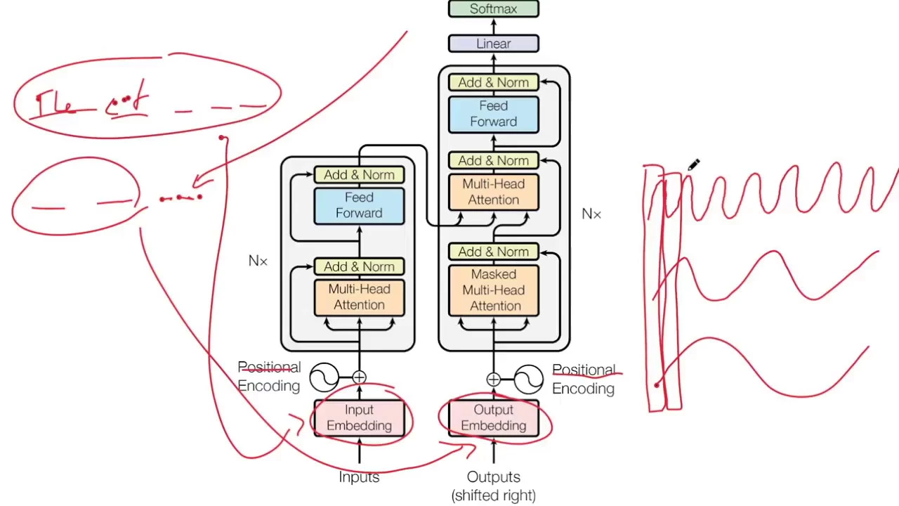
To realize this, the paper introduces the Transformer architecture. Although it retains an encoder and a decoder block, Kilcher highlights a critical conceptual difference from traditional architectures: it does not process tokens sequentially through recurrent loops across time. Instead, the entire input sentence and the partial target sentence generated so far are fed into the network simultaneously in parallel. The encoder processes the full source sequence at once, the decoder attends across both the source embeddings and its own representations, and the network immediately produces output probabilities over the vocabulary for the next token.

This fundamentally alters the mechanics of training and backpropagation. Under traditional RNNs, an entire sentence-to-sequence translation represents a single training unit that requires backpropagating through time (BPTT) across every sequential step. In the Transformer, predicting each token position operates as an independent step where the entire computation and backward pass happen all at once, without unrolling states over time. Kilcher underscores how radical this departure felt to the NLP community:

> “And this is kind of a paradigm shift in sequence processing because people were always convinced that you kind of need these recurrent things in order to to make good to learn these dependencies, but here they basically say: 'No, no, no, we can just do attention over everything and it will actually be fine.'”

[13:30](https://www.youtube.com/watch?v=iDulhoQ2pro&t=810s) Embeddings and Positional Encoding via Trigonometric Functions

The architecture begins symmetrically on both sides with standard input embeddings and output embeddings, mapping input tokens into continuous word vectors. Because the model completely removes recurrence and convolutions, it discards the sequential nature inherent to traditional recurrent algorithms. Without sequential step-by-step processing, the network needs an explicit mechanism to know the ordering of the words—identifying whether a specific word is at the beginning or the end of a sentence, or determining which of two words appears first.

```mermaid flowchart LR accTitle: Positional Encoding Overview accDescr: Diagram showing tokens embedded into vectors, combined with sinusoidal positional encodings across multiple frequencies, and fed into the Transformer blocks. subgraph Inputs["Input Processing"] A["Input Tokens"] --> B["Word Embeddings"] C["Sinusoidal Positional Encodings\n(Multiple Frequencies)"] --> D["Sum: Word + Position"] B --> D end D --> E["Transformer Attention Blocks"] ```

To encode order without recurrence, the architecture relies on trigonometric functions (sine and cosine waves) across varying frequencies. A slow sine wave can span the whole sequence, while faster sine waves oscillate rapidly. Across these differing wave scales, each sequence index receives a unique profile—acting as a continuous version of binary encoding. For instance, the first position might be evaluated as "down" across all waves, the second as "down-down-up," and the third as "up-down-up." When the network needs to compare two words, it checks their values across these sinusoidal scales: if their values match on a long, slow wave but differ on a fast wave, the network determines they are close together and resolves their precise relative order.

- Word tokens are converted to embedding vectors symmetrically on the input and output sides. - Positional encodings provide the network with word order awareness without using recurrence. - Multiple sinusoidal frequencies form a continuous analog to binary positional representation. - While the positional encodings give the model an important performance boost, Yannic notes they are secondary: “it's not that the meat of the thing.”

---

[16:02](https://www.youtube.com/watch?v=iDulhoQ2pro&t=962s) The Three Forms of Attention in the Transformer

The core innovation of the architecture is how it applies attention at three distinct locations in the network. The first application appears at the bottom-left of the diagram, where self-attention is computed directly over the input sentence. Here, the network creates a hidden representation of the entire input sequence all at once, choosing which input words to focus on or associate with one another. The second application is at the bottom-right, performing self-attention over the output sentence generated so far to build a target-side hidden state.

```mermaid flowchart TD accTitle: Transformer Attention Connectivity accDescr: Visual mapping of the three attention modules showing input self-attention, masked target self-attention, and the cross-attention mechanism bridging the encoder and decoder. subgraph Encoder["Encoder Stack"] Inp["Input Embeddings"] --> EncAtt["Input Self-Attention"] EncAtt --> Repr["Encoder Representation"] end

subgraph Decoder["Decoder Stack"] Tgt["Target Embeddings\n(Shifted Right)"] --> DecAtt["Target Self-Attention\n(Masked)"] DecAtt --> DecRepr["Target Representation"] end

subgraph CrossAttention["Encoder-Decoder Cross-Attention"] Repr -->|"Keys (K)"| XAtt["Cross Multi-Head Attention"] Repr -->|"Values (V)"| XAtt DecRepr -->|"Queries (Q)"| XAtt XAtt --> UpperLayers["Upper Feed-Forward & Output Layers"] end ```

The third, located at the top-right of the decoder stack, is the cross-attention mechanism that bridges the encoder and decoder. Yannic highlights this as the centerpiece of the system: “the top right is the most interesting part of the attention mechanism here where basically it unites the kind of encoder part with the kind of... it combines the source sentence with the target sentence that you've produced so far.” In this module, three separate connections feed into the multi-head attention block: two connections (the keys and the values) arrive directly from the encoder's source sentence representation, while the third connection (the query) comes up from the decoder's representation of the target sentence produced up to that point.

- **Bottom-left attention:** Self-attention over the input tokens to construct source representations all at once. - **Bottom-right attention:** Self-attention over target tokens generated so far. - **Top-right attention:** Cross-attention connecting the source and target representations. - Three incoming paths feed the cross-attention block: Keys ($K$) and Values ($V$) from the encoder, and Queries ($Q$) from the decoder.

---

[18:22](https://www.youtube.com/watch?v=iDulhoQ2pro&t=1102s) Dot-Product Attention as Soft Memory Addressing

The interaction inside the cross-attention module can be understood through the lens of an associative database or key-value retrieval table. The encoder discovers salient properties of the source sentence and outputs sets of keys ($K$) and values ($V$), while the decoder formulates queries ($Q$). In high-dimensional spaces, arbitrary vectors are generally close to orthogonal (roughly 90 degrees apart), meaning their dot product sits near zero. However, when a query aligns with a key, their dot product grows large.

$$\text{Attention}(Q, K, V) = \text{softmax}\left(\frac{Q K^T}{\sqrt{d_k}}\right)V$$

To turn these alignment scores into a selection mechanism, the network applies a softmax over the dot products. The softmax exponentiates each dot product, causing the largest value to dominate, and normalizes across the entries:

$$\text{Softmax}(x)_i = \frac{e^{x_i}}{\sum_{j} e^{x_j}}$$

This acts as a differentiable approximation of the $\max$ function. Multiplying the resulting probability distribution across the values selectively retrieves the value corresponding to the best-matching key.

```mermaid flowchart TD accTitle: Scaled Dot-Product Attention Flow accDescr: Step-by-step mathematical flow of computing queries and keys dot product, exponentiating via softmax, and taking a weighted sum of values. Q["Query (Q)\n(from Decoder)"] --> Dot["Dot Product (Q · K)"] K["Keys (K)\n(from Encoder)"] --> Dot Dot --> SMax["Softmax\n(Differentiable Max)"] SMax --> Weight["Attention Weights\n(Soft Distribution)"] V["Values (V)\n(from Encoder)"] --> Mult["Weighted Sum of Values"] Weight --> Mult Mult --> Out["Retrieved Representation"] ```

To illustrate this intuitively, Yannic presents an analogy of human attributes: the values are the actual data (such as a person's specific name, tallness, or weight), the keys serve as the indexing tags (labeled "name," "height," or "weight"), and the decoder query specifies what detail it needs (such as asking for the "name"). When the query aligns with the "name" key, the softmax selects that entry and returns the corresponding name value. While noting that the idea borrows conceptually from earlier work on differentiable neural computers and neural Turing machines, Yannic remarks: “it's a pretty ingenious it's not entirely new because it has been done of course before with all the differentiable Turing machines and whatnot but it's pretty cool that this actually works and actually works kind of better than RNNs if you simply do this.”

- Multi-head attention uses parallel sets of projection heads rather than a single vector. - Vector dot products quantify alignment; orthogonal vectors score near zero, aligned vectors yield large positive numbers. - Softmax exponentiates alignment scores, heavily weighting the maximum match while preserving end-to-end differentiability. - Multiplying the softmax distribution by the value matrix softly extracts the addressed information.

---

[25:50](https://www.youtube.com/watch?v=iDulhoQ2pro&t=1550s) Reducing Path Lengths and Improving Efficiency

The core theoretical justification for why attention outperforms recurrent architectures lies in path lengths for signal propagation. In recurrent neural networks, information must travel step-by-step through a long sequence of sequential state updates, where each intermediate transition introduces a chance to dilute or lose information. Attention collapses this distance by allowing direct, single-step connections between any two positions regardless of how far apart they sit in the sequence:

> “Basically that the point they make about this attention is that it reduces path lengths and kind of that's the the main reason why it should work better with this entire attention mechanism you reduce the amount of computation steps that information has to flow from one point in the network to another and that what brings the major improvement because all the computation steps can make you lose information and you don't want that you want short path lengths and so that's that's what this method achieves and they claim that's why it's better and it works so well.”

By minimizing the computational hops required across sequence positions, the Transformer preserves context far more effectively, leading to state-of-the-art results across machine translation and other benchmark experiments.

- Sequential recurrent models force signals through $O(n)$ transition steps, increasing the risk of information loss. - Pure attention mechanisms yield $O(1)$ path lengths between any arbitrary token pairs. - Shorter paths ensure gradients and semantic information propagate directly and efficiently across the entire context window.

[26:47](https://www.youtube.com/watch?v=iDulhoQ2pro&t=1607s) Concluding Thoughts and GitHub Codebase

Wrapping up his walkthrough of the state-of-the-art results established by the paper, Yannic Kilcher decides to bring the presentation to a close. For anyone looking to explore the implementation hands-on or experiment with the model directly, he points viewers to the authors' open-source materials, noting: “If you want to check it out yourself, they have extensive code on GitHub where you can build your own Transformer networks.” With that recommendation in place, he bids his audience farewell with a relaxed, cheerful sign-off wishing everyone a nice day.

- The authors provide extensive reference code publicly on GitHub, enabling researchers and developers to construct and train custom Transformer architectures.

## Mentioned Attention Is All You Need, Google, Transformer, Yannic Kilcher, Ashish Vaswani, Noam Shazeer, Niki Parmar, Jakob Uszkoreit, Llion Jones, Aidan N. Gomez, Lukasz Kaiser, Illia Polosukhin, Neural Turing Machines, GitHub, WMT 2014 English-to-German, WMT 2014 English-to-French

## Video description https://arxiv.org/abs/1706.03762

Abstract: The dominant sequence transduction models are based on complex recurrent or convolutional neural networks in an encoder-decoder configuration. The best performing models also connect the encoder and decoder through an attention mechanism. We propose a new simple network architecture, the Transformer, based solely on attention mechanisms, dispensing with recurrence and convolutions entirely. Experiments on two machine translation tasks show these models to be superior in quality while being more parallelizable and requiring significantly less time to train. Our model achieves 28.4 BLEU on the WMT 2014 English-to-German translation task, improving over the existing best results, including ensembles by over 2 BLEU. On the WMT 2014 English-to-French translation task, our model establishes a new single-model state-of-the-art BLEU score of 41.0 after training for 3.5 days on eight GPUs, a small fraction of the training costs of the best models from the literature. We show that the Transformer generalizes well to other tasks by applying it successfully to English constituency parsing both with large and limited training data.

Authors: Ashish Vaswani, Noam Shazeer, Niki Parmar, Jakob Uszkoreit, Llion Jones, Aidan N. Gomez, Lukasz Kaiser, Illia Polosukhin

[Source](https://www.youtube.com/watch?v=iDulhoQ2pro)

中文简报

谷歌摒弃循环神经网络,推出全注意力机制Transformer模型 用直接注意力取代逐步循环转换,将计算路径长度缩短至单次操作,在消除序列信息损失的同时实现序列的并行训练。 Kilcher概述了传统序列到序列循环神经网络的局限性,特别是其顺序瓶颈、容易出现长距离依赖衰减以及反向传播期间的展开约束。他解释了Transformer架构如何通过并行处理整个序列,并用正弦位置编码和三种专门的注意力操作取代循环,从而彻底革新了序列转换任务。聚焦于交叉注意力模块,Kilcher展示了缩放点积注意力如何对键、值和查询充当可微的内存检索机制。最终,他强调将信息流的路径长度从顺序跳步压缩至单步,是该架构取得最先进翻译性能的核心概念驱动力。 Vaswani等人提出了Transformer,这种架构完全摒弃了循环神经网络和卷积,完全依靠序列间的纯注意力机制。 (10:33) 通过用直接注意力连接取代循环转换,Transformer将任意标记之间的信息路径长度减少为单步操作,从而缓解了传统RNN严重的信号衰减问题。 (25:50) Transformer不再跨时间步进行顺序循环,而是同时处理整个源序列和目标序列,消除了反向传播期间的顺序展开。 (10:33) 在翻译基准测试中,该模型创下了最先进的成绩(WMT 2014英德翻译为28.4 BLEU,英法翻译为41.0 BLEU),同时所需的训练成本显著降低。

Reading summary

In his review of Google's paper "Attention Is All You Need," Yannic Kilcher explains the authors' central thesis: natural language processing models should discard recurrent neural networks (RNNs) entirely. By substituting sequential recurrence with attention across whole sequences simultaneously, the Transformer architecture eliminates the long-range dependency bottlenecks that constrain traditional sequence-to-sequence translation. Recurrent Bottlenecks and Long-Range Dependency Failures (0:00) Traditional sequence-to-sequence machine translation relies on an encoder-decoder framework utilizing recurrent networks such as RNNs or LSTMs. The encoder processes input text token by token, updating an internal hidden state through a recurrent transition function where each state depends on the previous hidden state and the current word vector. Under this formulation, the final encoder hidden state must compress the entire semantic meaning of the source sentence into a single vector bridge before passing it to the decoder, which unpacks the representation token by token. Kilcher highlights that this setup creates a severe vulnerability for long-range dependencies. In real-world translation, where syntax and word order frequently shift, words appearing early in a source sequence must traverse a lengthy cascade of encoder transitions and initial decoding steps before influencing later outputs. This extended sequential path makes it difficult for networks to retain early semantic nuances, as each intermediate computation step introduces opportunities to dilute or lose critical information. Parallel Sequence Processing and Collapsed Path Lengths (10:33) The Transformer architecture departs from this paradigm by eliminating recurrent loops and convolutions altogether. Instead of unrolling states sequentially over time, the network ingests the entire source sentence and the partial target sentence simultaneously. This architectural shift enables parallel computation across tokens during training, replacing backpropagation through time across sequential steps with independent token predictions across the vocabulary. According to Kilcher, the primary theoretical justification provided by the authors is the drastic reduction in signal path length. Recurrent models force information to travel through a long sequence of intermediate transitions, creating a persistent risk of degradation. In contrast, pure attention mechanisms achieve direct connections between any arbitrary pair of tokens regardless of their sequence positions. Collapsing this computational distance allows gradients and semantic context to flow directly across the entire sequence window without being filtered through intervening time steps. Reconstructing Word Order with Sinusoidal Signals (13:30) Because the Transformer processes tokens simultaneously rather than sequentially, it discards the implicit order inherent to recurrent algorithms. To identify whether a word appears at the start, middle, or end of a sequence—or to determine which of two words comes first—the model supplements word embeddings with sinusoidal positional encodings derived from trigonometric functions across varying frequencies. These encodings function as a continuous analog to binary representations. Slower sine waves span the entire sequence, while higher-frequency waves oscillate rapidly. When evaluating tokens, the network compares values across these frequency scales: matching values on low-frequency waves combined with differences on high-frequency waves signal that two words sit close to one another, establishing their relative positions. Although Kilcher views this mechanism as secondary to the core attention mechanism, it provides the ordering context essential for sequence parsing. Tripartite Attention as Differentiable Memory Retrieval (16:02) The Transformer applies attention across three distinct locations: self-attention over the source sequence to construct input representations, self-attention over previously emitted target tokens, and a cross-attention module connecting encoder representations to the decoder stack. Kilcher identifies this cross-attention block as the system's centerpiece, where keys and values generated by the encoder are queried by the decoder. This interaction operates like soft associative memory addressing. The decoder produces a query vector, which is compared against encoder keys via dot products. Because orthogonal vectors yield near-zero dot products while aligned vectors produce large values, the dot product quantifies alignment. A softmax function then exponentiates and normalizes these scores, acting as a differentiable approximation of a maximum selection function. Multiplying the resulting probability distribution across the value vectors softly retrieves the most relevant semantic data in a single step. Kilcher summarizes that by discarding recurrent connections in favor of direct, multi-head attention addressing, the Transformer established new state-of-the-art benchmarks in machine translation. To support ongoing adoption and experimentation across the machine learning community, the original authors made their implementation code publicly available on GitHub.

精炼阅读摘要

Yannic Kilcher 在对论文《Attention Is All You Need》的解读中指出,该研究主张自然语言处理应彻底摒弃循环神经网络(RNN),仅依靠全序列并行注意力和位置编码即可高效建模长距离依赖。 传统循环模型的传递瓶颈与长程依赖困境 (0:00) 在传统的序列到序列(seq2seq)机器翻译任务中,标准 RNN 或 LSTM 编码器按时间步逐个处理源序列词元,将每个词向量与前一隐状态 $h_{t-1}$ 结合以输出新的隐状态 $h_t$。整句的语义最终必须压缩进单一向量(例如四词元序列中的 $h_4$),再移交给解码器逐步解压并生成目标语言词元。Kilcher 解释称,解码器严重依赖隐状态来捕捉全句语义,同时以先前生成的词引导局部语法与语句连贯性。 这种级联结构在处理句首出现的词元时极度脆弱。若解码器后续需要翻译先前的词元,相关信息必须经过漫长的编码与解码状态转移链条传递,导致长距离依赖难以学习。虽然早期引入的注意力机制通过允许解码器生成键或查询直接索引编码器隐状态,以此缩短了信息传输路径,但整个网络的核心骨干依然受困于逐步递推的循环计算中。 彻底舍弃循环机制:Transformer的并行范式转换 (10:33) Google 论文的核心论点在于循环计算并非不可或缺,研究人员完全可以在全序列上直接并行应用注意力机制。Transformer 架构虽然保留了解码器和编码器的结构划分,但彻底移除了时间维度的循环循环。源序列和已生成的目标序列被同时输入网络,编码器一次性处理完整源句,并在词表上直接计算下一词元的概率分布。 这种设计从根本上改变了模型的训练与反向传播机制。传统的 RNN 翻译需要跨越全部时间步展开并执行沿时间反向传播(BPTT),而 Transformer 预测每个词元位置都是一次独立的并行计算步骤。Kilcher 强调,自然语言处理界此前普遍认为必须依靠循环机制来捕捉上下文依赖,而该论文证明直接在大局上计算注意力不仅可行,而且大幅颠覆了原有的序列建模思维。 三角函数位置编码:无循环下的顺序表示方案 (13:30) 由于 Transformer 完全剔除了循环与卷积结构,模型失去了天然的时序感知能力,因此必须引入显式机制来识别词元在句中的相对与绝对顺序。该架构在输入端与输出端对称地保留了词嵌入,并通过向词向量中叠加基于正弦与余弦函数的多频率位置编码来弥补顺序信息的缺失。 这种三角函数编码覆盖了从低频到高频的不同波长,慢速波跨越整句,而快速波则高频振荡,在多尺度下为每一个序列索引生成独一无二的波峰波谷组合,其逻辑类似于连续形式的二进制编码。网络通过比对词元在长波与短波上的数值,便能精准判断两词间的距离与前后相对顺序。虽然 Kilcher 认为位置编码只是辅助组件而非核心本质,但它为无循环并行模型提供了至关重要的时序分辨能力。 三类注意力结构与点积软内存寻址机理 (16:02) Transformer 内部部署了三处注意力机制:编码器底部的输入自注意力(一次性构建源序列表示)、解码器底部的掩码目标自注意力(处理已生成的目标词元),以及解码器上方的编码器-解码器交叉注意力。Kilcher 指出,交叉注意力是架构中最关键的枢纽,它接收来自编码器的键(Keys, $K$)与值(Values, $V$),并与解码器生成的查询(Queries, $Q$)交互,实现了源句与目标句表示的深度融合。 该模块的数学计算将注意力视作连续可微的联想数据库寻址机制。在高维空间中,不相关的向量往往近似正交且点积接近零,而匹配的查询与键则会产生较大的正点积。通过对除以缩放因子的点积矩阵计算 Softmax,网络生成了近似于最大值选取的概率分布权重,再与值矩阵相乘完成信息提取。Kilcher 借用人类特征的类比解释这一过程:键犹如“姓名”或“身高”的索引标签,值是具体的数据,解码器发出针对特定标签的查询,模型便通过点积匹配柔性提取出对应的值。 信号传播路径压缩带来的理论与效率优势 (25:50) 根据论文给出的理论解释,纯注意力架构击败循环模型的根本原因在于极大地压缩了信号传播的路径长度。在传统循环神经网络中,任意两个远距离词元之间的信息交换都必须穿透 $O(n)$ 步状态转换,每一步计算都存在稀释、扭曲或丢失上下文语义的风险。 相比之下,注意力机制在任意词元对之间建立了单步可达的直接连接,将路径长度缩短至 $O(1)$。这种直接的信息流动使梯度反向传播和语义特征提取都不再受制于序列长度,显著降低了长文本中的遗忘风险。论文作者主张,正是计算跳数的最小化让 Transformer 在机器翻译等基准测试中刷新了多项纪录并取得了优异的性能表现。 Kilcher 总结指出,论文作者在 GitHub 上开源了完整的 Transformer 代码库以供研究者构建和训练模型。该架构证明了完全移除循环连接的可行性,通过更短的计算路径和全局注意力重新定义了序列建模的基准范式。

Detailed notes — zh

## Background 该视频由机器学习研究者 Yannic Kilcher 于 2017 年 11 月 28 日发布在 YouTube 平台上。视频简介提供了论文《Attention Is All You Need》(arXiv:1706.03762)的链接、摘要以及 Google 团队等作者名单,展示了完全基于注意力机制、彻底摒弃循环与卷积的 Transformer 架构及其在机器翻译任务上取得的突破性成果。 ## TL;DR Yannic Kilcher 深入剖析了革命性论文《Attention Is All You Need》的核心突破,详细拆解了为什么序列建模应当彻底抛弃传统的 RNN 与 LSTM。他对比了传统 Seq2Seq 架构受制于 $O(N)$ 逐步递归而产生的长程依赖瓶颈与语义稀释,进而阐述了 Transformer 如何借助位置编码与全并行前向计算实现范式转移。视频重点解析了自注意力、交叉注意力的代数运算与几何意义,用生动的“属性字典”和可微寻址比喻讲透了 Query、Key、Value 的匹配机制,并指出极大缩短信息传递路径与高并行性正是 Transformer 全面刷新 SOTA 的关键所在。 ## Atmosphere & style 讲解风格兼具学术严谨与黑板式手绘的随性洒脱,Yannic 操着一口标志性的口音,在屏幕上随笔勾勒波形图、矩阵与直观示意图,将晦涩的线性代数与几何概念化繁为简。整个视频充满技术洞察的兴奋感与顿悟感,既有抽丝剥茧拆解核心机制的深度思考,又保持着轻松流畅、条理分明的讲述节奏,让观众切实体会到见证一场深度学习范式革命的纯粹智力乐趣。 ## Bulletin - [00:00](https://www.youtube.com/watch?v=iDulhoQ2pro&t=0s) Google 团队提出 Transformer 架构,彻底摒弃传统序列建模中依赖的循环神经网络(RNN)与卷积,仅依靠自注意力机制即可实现高质量的序列转换。 - [23:32](https://www.youtube.com/watch?v=iDulhoQ2pro&t=1412s) Transformer 将任意两个词元间的信息交互路径从传统 RNN 的 O(N) 线性距离大幅缩短至 O(1),从而彻底解决了序列建模中的长程依赖与梯度信息丢失瓶颈。 - [10:33](https://www.youtube.com/watch?v=iDulhoQ2pro&t=633s) 在训练效率上,Transformer 摆脱了 BPTT 的时间步串行依赖,实现全并行单步前向与反向计算;在 WMT 2014 英德翻译上达到 28.4 BLEU,英法翻译仅需 8 块 GPU 训练 3.5 天便创下 41.0 BLEU 的 SOTA 记录。 - [13:30](https://www.youtube.com/watch?v=iDulhoQ2pro&t=810s) 架构引入多频率正弦波位置编码来补偿全并行计算下丢失的词序几何信息,并采用类似字典查找的 Query-Key-Value 可微点积注意力机制实现精准的动态语义寻址。 ## Key takeaways - [00:00](https://www.youtube.com/watch?v=iDulhoQ2pro&t=0s) 传统 Seq2Seq 架构依赖 RNN/LSTM 进行逐步循环编码,所有历史语义信息被强制压缩入单一隐藏状态向量,极易出现信息稀释与梯度衰减。 - [05:06](https://www.youtube.com/watch?v=iDulhoQ2pro&t=306s) RNN 在解码生成时面临长程依赖难题,目标端预测词与源句子关键动词之间的信息传递路径随序列长度线性增加,难以学习复杂语法打乱的跨语言映射。 - [07:30](https://www.youtube.com/watch?v=iDulhoQ2pro&t=450s) 早期注意力机制通过引入动态键值加权寻址缩短了信息路径,但仅被当作传统循环网络的外挂辅助,未完全释放其潜力。 - [10:33](https://www.youtube.com/watch?v=iDulhoQ2pro&t=633s) 《Attention Is All You Need》提出核心范式转移:彻底废除循环结构,仅依靠注意力机制即可完成序列全局上下文依赖的建模。 - [11:10](https://www.youtube.com/watch?v=iDulhoQ2pro&t=670s) Transformer 采用全并行单步计算模式,整条源序列与已生成目标序列一次性输入网络,避开了代价高昂的时间反向传播(BPTT)。 - [13:30](https://www.youtube.com/watch?v=iDulhoQ2pro&t=810s) 因抛弃了循环的时序传递,模型必须使用多尺度正弦与余弦函数的位置编码,作为连续二进制坐标将绝对和相对词序信息重新注入词嵌入中。 - [16:05](https://www.youtube.com/watch?v=iDulhoQ2pro&t=965s) 网络内部协同运行三种注意力:编码器自注意力用于源句语义提炼,带掩码的解码器自注意力用于自回归防穿越,跨注意力则连接源端与目标端。 - [17:30](https://www.youtube.com/watch?v=iDulhoQ2pro&t=1050s) 右上角跨注意力(Cross-Attention)结构中,编码器输出对应键(Keys)和值(Values),解码器输出对应查询(Queries)。 - [18:54](https://www.youtube.com/watch?v=iDulhoQ2pro&t=1134s) 缩放点积注意力通过计算 Query 与 Key 的向量夹角对齐度,利用 Softmax 的指数放大效应实现可微分的近邻查表与记忆检索机制。 - [23:32](https://www.youtube.com/watch?v=iDulhoQ2pro&t=1412s) Query、Key、Value 的关系类似于字典查询:Values 代表具体属性内容,Keys 代表索引标签,Queries 代表解码器当前需要主动检索的特征要求。 - [25:00](https://www.youtube.com/watch?v=iDulhoQ2pro&t=1500s) Transformer 取得压倒性优势的本质在于将任意两点间的长途信息传递步数直接压缩至一步(短路径效应),显著降低了深层传递中的语义耗损。 - [26:47](https://www.youtube.com/watch?v=iDulhoQ2pro&t=1607s) 论文所有实现及核心网络构建方法已在 GitHub 完全开源,推动了后续 NLP 与多模态基础模型的飞速发展。 ## Detailed walkthrough ### [00:00](https://www.youtube.com/watch?v=iDulhoQ2pro&t=0s) 告别循环神经网络:Seq2Seq 范式与传统 RNN 机制 Yannic Kilcher 开篇明确指出,虽然他最近连续讲了几篇 Google 的论文,但他并不为 Google 工作,纯粹是因为这篇论文极具突破性。这篇名为《Attention Is All You Need》的论文核心主张非常激进:在序列处理(尤其是自然语言处理)领域,我们应当彻底抛弃传统的循环神经网络(RNN)。 以经典的机器翻译为例,假设我们要将英文句子 “the cat eats the mouse” 翻译成德语。在传统自然语言处理的 Sequence-to-Sequence(Seq2Seq)任务中,标准做法是将源语言句子整体编码成某种内部表征,通常是一个固定维度的隐状态向量,再由解码端将该向量重新展开还原为目标语言。过去这类任务几乎完全由 RNN 或 LSTM(长短期记忆网络)主导。 在传统的 RNN 编码过程中,模型按时间步逐词遍历源句子。以第一个词 “the” 为例,模型首先将其映射为一个词向量(word vector),然后送入编码器神经网络函数,结合初始隐状态(通常全零初始化或可学习)计算得到当前步的隐藏状态 $h_0$。随后取下一个词 “cat”,将其词向量和上一步的隐藏状态 $h_0$ 同时喂入**同一个**编码器网络函数,计算出新的隐藏状态 $h_1$。依此类推,网络依次生成 $h_2$、$h_3$ 直至最后一个词的隐状态 $h_4$。 在解码阶段,编码器输出的最后一个隐藏状态 $h_4$ 会以类似的方式注入解码器网络。解码器每一步吐出一个目标语言单词并更新隐藏状态(如输出目标词与 $h_5$),接着将新状态 $h_5$ 与刚刚生成的单词再次输入解码器,迭代预测下一个词。 ```mermaid flowchart LR accTitle: 传统 RNN 编码解码架构 accDescr: 展现传统 RNN 逐词递归编码并在解码端串行展开的 Seq2Seq 流程 subgraph ENC ["编码端 (Encoder)"] direction LR W0["the"] --> E0["Encoder"] W1["cat"] --> E1["Encoder"] W2["eats..."] --> E2["Encoder"] E0 -->|"h0"| E1 E1 -->|"h1"| E2 end subgraph DEC ["解码端 (Decoder)"] direction LR D0["Decoder"] -->|"h5, 词1"| D1["Decoder"] D1 -->|"h6, 词2"| D2["Decoder"] end E2 -->|"h4"| D0 ``` - 隐藏状态负责压缩整句话的全局语义信息,而解码器每步重新吃进上一个输出词,则是为了保证局部语法的连续性与合规性。 - 整个架构的核心递归式为:当前隐藏状态 $h_t = f(h_{t-1}, x_t)$,其中函数 $f$ 在每个时间步严格共享权重参数。 --- ### [05:06](https://www.youtube.com/watch?v=iDulhoQ2pro&t=306s) 传统架构的致命痛点:长程依赖与注意力机制的引入 当解码器试图预测德语词汇时,传统 RNN 面临极为苛刻的信息传输路径。假设解码器当前需要输出对应于英文中 “eats” 的动作词,但解码器此时能拿到的唯一输入仅仅是上一时间步生成的德语词以及当前的隐藏状态 $h_6$。这意味着,“eats” 这个词的语义信息必须历经漫长的漂流:首先被编码成词向量,通过一次通用编码器函数,随后被连续多步的隐藏状态不断压缩混合,最后再在解码端跨越数个时间步传递下来。 隐藏状态被强行要求同时背负所有历史词汇的语义、语序以及整句的句法结构,这导致信息在传递链路中发生严重稀释或丢失。Yannic 强调:“so it's very hard for an RNN to learn all of this what they what we call long-range dependencies”。人类语言无法直接做简单的一对一词汇直译,因为目标语言的语序经常被重新打乱,甚至一个词会扩展成多个词或完全不同的句式结构。 为了解决长程依赖瓶颈,研究者引入了注意力机制(Attention Mechanism)。注意力机制赋予了解码端主动向后回溯、直接检索输入序列特定区域的能力。在预测特定动作时,解码器不再只依赖单一的状态向量,而是直接把注意力投射到编码 “eats” 时的对应隐藏状态上。通过类似神经图灵机(Neural Turing Machine)的寻址策略,解码器在当前时间步生成一系列查询键(Keys)$K_1$ 到 $K_n$,通过 Softmax 归一化对各个编码步的隐状态进行加权寻址,以极短的信息路径直接提取源句中的关键特征。 - 传统 RNN 的信息路径长度随序列长度线性增加($O(N)$),而注意力机制将路径缩短至一步直达,极大缓解了长距离梯度消失与语义衰减。 - 解码器在此扮演了主动查询者的角色,通过加权平均机制从编码端提取最相关的隐藏状态子集。 --- ### [10:33](https://www.youtube.com/watch?v=iDulhoQ2pro&t=633s) 彻底摒弃循环:Transformer 的范式转移与并行单步计算 尽管带有注意力的 RNN 取得了显著成功,但这篇论文的作者们做出了惊人断言:既然注意力机制如此强大,那我们何必还要保留底层的循环网络呢?Yannic 总结道:“they basically say attention is all you need you don't need the entire recurrent things”。作者提出了一种全新的网络架构——Transformer,彻底废弃了时间递归结构。 Transformer 虽然在逻辑上依然保留了编码器(Encoder)与解码器(Decoder)两大部分,但它的运行方式与 RNN 有着本质区别。在 Transformer 中,所有操作均是全并行一次性完成的(“it all happens at once”)。以当前预测第三个词为例,系统直接将**整条源句子**一次性送入编码器模块,同时将**截至目前已生成的所有目标词序列**一次性送入解码器模块。 ```mermaid flowchart TD accTitle: Transformer 宏观训练与推理架构 accDescr: 展现源序列与目标前缀并行输入 Transformer 编码器与解码器并输出下一词概率的流程 subgraph IN ["输入层 (Inputs)"] SRC["整条源句子序列"] TGT["已生成的全部目标前缀"] end subgraph TR ["Transformer 架构"] ENC["Encoder (多层自注意力+FFN)"] DEC["Decoder (Masked自注意力+交叉注意力)"] end SRC --> ENC ENC --> DEC TGT --> DEC DEC --> PROB["输出词表概率分布 (下一词)"] ``` 在网络最终的输出端,模型通过全连接层计算出目标词表的概率分布,直接选出最高概率的词作为下一个输出,随后更新序列并重复这一过程。这就带来了序列建模范式的根本性转变: 在传统 RNN 中,整个句对的翻译构成了单次样本训练单元,误差必须沿着时间序列一步一步沿反向传播(Backpropagation Through Time, BPTT);而在 Transformer 中,生成单个 Token 的预测即为一个完全独立的训练样本前向/反向过程,所有的自注意力计算均在单次前向传递中并行展开。 正如 Yannic 所评论的那样,这是序列处理领域的一场深刻变革:“and this is kind of a paradigm shift in sequence processing because people were always convinced that you kind of need these recurrent things in order to to make good to learn these dependencies”。长久以来研究界普遍坚信必须依赖循环单元才能捕获上下文依赖,而该论文证明,仅依靠全局注意力机制就能更加出色地完成任务。 - **消除时序递归**:去除了隐藏状态在时间轴上的显式链式依赖,模型可以直接对序列中的任意两个位置建立直接联系。 - **单步完整计算**:反向传播仅针对当前步的所有并行连接展开,无需进行高计算开销的跨时间步递归梯度回传。 ### [13:30](https://www.youtube.com/watch?v=iDulhoQ2pro&t=810s) 位置编码:基于三角函数的连续二进制表征 在彻底摒弃了循环神经网络(RNN)和卷积网络(CNN)之后,模型在一次性并行吃进所有词向量时,必须解决一个致命的缺陷:模型完全丢失了序列的顺序信息。Yannic Kilcher 指出,输入嵌入(Input Embedding)和输出嵌入(Output Embedding)是完全对称的,词元(tokens)直接被映射为词向量。然而,“因为你的算法丢失了这种序列性质,你必须对这些通过网络的单词所在的位置进行编码”,这样网络才能辨别出“啊哈,这是一个句首的词,还是一个句尾的词”,或者能够对比两个词中“哪一个在前,哪一个在后”。 ```mermaid flowchart LR accTitle: Positional Encoding Mechanism accDescr: Visualizing how sinusoidal waves of different frequencies create continuous positional vectors for words in a sequence. subgraph Waves["不同频率的正弦波 (Sinusoidal Waves)"] W1["低频长波 (判断全局远近)"] W2["中频波"] W3["高频短波 (判断局部相邻与先后)"] end subgraph Pos["位置向量 (Positional Vector)"] P1["位置 1: [低, 低, 低...]"] P2["位置 2: [低, 低, 高...]"] P3["位置 3: [高, 低, 高...]"] end Waves --> P1 Waves --> P2 Waves --> P3 ``` 为了让网络轻松处理位置关系,论文采用了基于三角函数的编码方式。Yannic 在屏幕上画出了多条波长各异的正弦波——从变化缓慢的长波,到振荡极快的短波。他解释道,这本质上是“位置二进制编码的一种连续版本”: - 序列中的第一个位置可能在所有波形上都处于低位(“all down”); - 第二个位置可能呈现为“低-低-高”(down down up); - 第三个位置则变为“高-低-高”(up down up),以此类推。 通过观察这些多尺度波形上的取值,网络能够迅速对比任意两个词。如果一个词在长波上取高值,另一个在长波上取低值,模型便能立刻知道它们相距甚远,一个在句首,一个在句尾;而如果两个词在慢波上取值相近,网络再去观察高频快波,就能精确判定它们是否紧挨着,以及究竟“谁在前,谁在后”。Yannic 坦言,位置编码虽然能给网络带来显著的性能提升,但它并不是整个架构最核心的本质;真正的重头戏在于进入网络之后的注意力机制。 - 嵌入机制:输入与输出词向量采用对称的词嵌入投影(Word Embeddings)。 - 编码逻辑:利用不同频率的 $\sin$ 和 $\cos$ 函数生成连续多维向量,充当词序的时空坐标。 - 相对距离识别:长波用于捕捉宏观的全局距离,高频短波用于确定局部相对先后顺序。 --- ### [16:05](https://www.youtube.com/watch?v=iDulhoQ2pro&t=965s) 三种注意力机制与跨注意力连接结构 当嵌入向量与位置编码相加进入网络后,系统开始执行三种不同形态的注意力计算: 1. **左下角编码器自注意力(Encoder Self-Attention)**:直接在输入句子上进行注意力计算。网络不再像 RNN 那样逐步推导,而是一次性将整句压入隐层表示,本质上就是让输入序列在内部自由选择“该更多关注哪个词,更少关注哪个词”。 2. **右下角解码器自注意力(Masked Decoder Self-Attention)**:对截至目前已经生成的输出目标句进行编码,生成对应的隐状态表示。 3. **右上角交叉注意力(Cross-Attention)**:这是整个注意力机制中最精彩的部分,它将编码器部分与解码器部分融合在一起,连接了源句子与当前已生成的目标句子。 ```mermaid flowchart TD accTitle: Transformer Attention Cross Connection accDescr: Data flow into Multi-Head Cross-Attention from encoder and decoder representations. subgraph Enc["编码器端 (Source Sentence)"] SrcOut["源句子隐层表示"] end subgraph Dec["解码器端 (Target Sentence)"] TgtOut["目标句子已生成隐层表示"] end subgraph CrossAttn["右上角 Multi-Head Attention"] K["Keys (键)"] V["Values (值)"] Q["Queries (查询)"] end SrcOut -->|"连接 1"| K SrcOut -->|"连接 2"| V TgtOut -->|"连接 3"| Q ``` Yannic 擦掉图上的多余圈画,特别强调了右上角注意力模块的连线结构。进入这个多头注意力模块的一共有三根连接线:两根来自编码源句子的输出端,一根来自已生成输出的解码端。这三条连接精确对应着注意力机制的三大基石: - **键(Keys)**:由源句子的编码部分输出; - **值(Values)**:同样由源句子的编码部分输出; - **查询(Queries)**:由目标句子的已生成部分输出。 在 Multi-Head Attention(多头注意力)设计中,这类 Query、Key、Value 不止一组,而是同时存在多个并行子集,从多个特征子空间协同提取信息。 --- ### [18:54](https://www.youtube.com/watch?v=iDulhoQ2pro&t=1134s) 点积匹配、Softmax 索引与可微记忆寻址 Yannic 深入拆解了注意力的代数运算过程:首先计算查询(Queries)与键(Keys)的点积(Dot Product),对结果应用 Softmax 函数进行归一化,最后将其乘以值(Values)。 在几何与线性代数层面,高维空间中的两个向量的点积直接反映了两者的夹角。“尤其是在高维空间中,绝大多数随机向量彼此之间都趋近于 90 度垂直”,它们的点积接近于零;但如果某一个 Query 与某一个 Key 在方向上高度对齐,它们的点积就会非常大。 ```mermaid flowchart LR accTitle: Scaled Dot-Product Attention Flow accDescr: Computational pipeline of Queries and Keys dot product leading to Softmax and Value indexing. Q["Query (Q)"] & K["Keys (K)"] --> Dot["点积计算 (Dot Product: Q · K)"] Dot --> SM["Softmax 归一化 (指数放大 + 概率化)"] SM --> Mult["加权求和 (乘以 Values: V)"] V["Values (V)"] --> Mult Mult --> Out["注意力上下文输出"] ``` Yannic 打了个生动的比方:空间中散布着一堆 Keys 向量,每个 Key 在表格中都关联着一个 Value(如 Value 1、Value 2、Value 3、Value 4)。当引入一个 Query 向量时,系统计算该 Query 与所有 Keys 的点积: - **Softmax 运算**:对于输入数值 $x_1, \dots, x_n$,将其映射为 $e^{x_i}$ 并除以全量求和 $\sum e^{x_i}$。指数运算会把原本略微领先的较大数值无限放大,而让较小的数值趋于零,实现可微分的近似最大值选择(Argmax)。 - **可微寻址(Differentiable Memory Indexing)**:Softmax 产生一个尖锐的概率分布,其中与 Query 最对齐的 Key(例如 Key 2)权重接近 1,其余接近 0。以此概率分布与 Values 相乘,便能精准提取出 Value 2。这相当于一套在连续向量空间中工作的动态查表与记忆检索机制。 --- ### [23:32](https://www.youtube.com/watch?v=iDulhoQ2pro&t=1412s) 属性字典类比与缩短信息路径的优势 为了将这一套抽象的数学公式讲透,Yannic 用人类身份信息的“属性字典”进行了解释: - 源句子的编码器在句子中发现各种有趣的特征,并将它们打包成键值对(Key-Value pairs)。 - **Values(值)**:代表源句子里具体有趣的内容实体,好比一个人的具体属性——名字叫什么、身材有多高、体重是多少。 - **Keys(键)**:代表索引这些属性的标签或寻址方式,好比属性目录中的“姓名”、“身高”、“体重”索引词。 - **Queries(查询)**:来自目标句子的生成端,它主动发问:“我现在需要特定的信息”。如果它当前的 Query 是“想要姓名”,该 Query 就会与 Key 里的“姓名”产生极高的对齐点积,从而把 Value 里面具体的“某某人名字”抽取出来,送入后面的网络层继续计算。 Yannic 赞叹道:“我认为这是一个非常精妙的设计。它并不是完全全新的东西,因为以前在可微图灵机(Differentiable Turing Machines)等研究中就已经尝试过类似思路,但令人惊叹的是它在这里切实起效了,而且仅仅依靠这种结构,表现就直接超越了 RNN。” 在讨论 Transformer 为什么能取得压倒性胜利时,Yannic 指出了论文的核心论点:缩短路径长度(Reducing Path Lengths)。“通过整套注意力机制,你减少了信息在网络中从一个节点传递到另一个节点所必须经历的计算步数,而这正是带来重大改进的关键所在,因为过多的计算步数会导致信息丢失,你绝不希望那样,你想要的是短路径。”在传统的 RNN 链条中,首尾信息传递需要经过等同于句子长度 $O(n)$ 步的逐步累加,极易遗忘;而自注意力机制仅需 $O(1)$ 的单一计算步即可连接任意两个词。正是这种短路径和高并行度,让 Transformer 在多项机器翻译实验中全面打破了历史纪录,建立了全新的 SOTA。 ### [26:47](https://www.youtube.com/watch?v=iDulhoQ2pro&t=1607s) 总结与开源代码资源 在完整剖析了论文的核心架构与各项前沿实验成果之后,Yannic Kilcher 准备结束整期讲解。他向想要亲自实践或深入研究的观众推荐了论文团队开源的代码仓库,指出作者团队在 GitHub 上提供了非常详尽的实现代码,开发者和研究人员可以直接利用这些资源来搭建属于自己的 Transformer 网络。 在视频的最后,Yannic 以标志性的轻松语气向观众告别,整篇论文的讲解也在轻快友好的氛围中落下帷幕。正如 Yannic Kilcher 所说:“and I think I will conclude here if you want to check it out yourself they have extensive code on github where you can build your own transformer networks and with that have a nice day and see ya.” - **开源实现**:作者团队在 GitHub 上发布了完备的代码库,支持用户复现并构建自定义的 Transformer 网络结构。 - **结语致意**:主讲人简短向观众致意道别,为整场论文精读画上句号。 ## Notable quotes > [10:33](https://www.youtube.com/watch?v=iDulhoQ2pro&t=633s) they basically say attention is all you need you don't need the entire recurrent things — Yannic Kilcher > [05:06](https://www.youtube.com/watch?v=iDulhoQ2pro&t=306s) so it's very hard for an RNN to learn all of this what they what we call long-range dependencies — Yannic Kilcher ## Mentioned Transformer, RNN, LSTM, Seq2Seq, Neural Turing Machine, Attention Mechanism, Self-Attention, Cross-Attention, Softmax, Google, Yannic Kilcher, Ashish Vaswani, Noam Shazeer, Niki Parmar, Jakob Uszkoreit, Llion Jones, Aidan N. Gomez, Lukasz Kaiser, Illia Polosukhin, WMT 2014 ## Video description https://arxiv.org/abs/1706.03762 Abstract: The dominant sequence transduction models are based on complex recurrent or convolutional neural networks in an encoder-decoder configuration. The best performing models also connect the encoder and decoder through an attention mechanism. We propose a new simple network architecture, the Transformer, based solely on attention mechanisms, dispensing with recurrence and convolutions entirely. Experiments on two machine translation tasks show these models to be superior in quality while being more parallelizable and requiring significantly less time to train. Our model achieves 28.4 BLEU on the WMT 2014 English-to-German translation task, improving over the existing best results, including ensembles by over 2 BLEU. On the WMT 2014 English-to-French translation task, our model establishes a new single-model state-of-the-art BLEU score of 41.0 after training for 3.5 days on eight GPUs, a small fraction of the training costs of the best models from the literature. We show that the Transformer generalizes well to other tasks by applying it successfully to English constituency parsing both with large and limited training data. Authors: Ashish Vaswani, Noam Shazeer, Niki Parmar, Jakob Uszkoreit, Llion Jones, Aidan N. Gomez, Lukasz Kaiser, Illia Polosukhin [Source](https://www.youtube.com/watch?v=iDulhoQ2pro)

Source quotes

[10:33] Yannic Kilcher: they basically say attention is all you need you don't need the entire recurrent things [5:06] Yannic Kilcher: so it's very hard for an RNN to learn all of this what they what we call long-range dependencies

Original transcript

[0:00] hi there today we're looking at [0:03] attention is all you need by Google just [0:06] to declare I don't work for Google just [0:08] because we've been looking at Google [0:10] papers lately but it's just an [0:12] interesting paper and we're gonna see [0:15] what's the deal with it so basically [0:18] what the authors are saying is we should [0:21] kind of get away from basically onions [0:27] so traditionally what you would do and [0:30] these authors particular interested in [0:33] NLP natural language processing so [0:35] traditionally when you had like a [0:37] language task the cat eats the mouse and [0:46] you would like to translate this to say [0:50] any other language like let's say German [0:56] or whatever what you would do is you [1:00] would try to encode this sentence into a [1:03] representation and then decode it again [1:05] so somehow somehow this sentence needs [1:10] to all go into say one vector and then [1:13] this one vector needs to somehow be [1:16] transformed into the target language so [1:20] these are tradition called sack to sack [1:22] tasks and they have been solved so far [1:27] using recurrent neural networks you [1:30] might know the Alice TN networks that [1:34] are very popular for these tasks what [1:36] basically happens in an RNN is that you [1:38] go over the say source sentence here one [1:42] by one here you take the word the you [1:45] kind of encode it maybe with a word [1:48] vector if you know that is so you turn [1:51] it into like a vector a word vector and [1:54] then you use a neural network to turn [1:57] this vector into what we call a hidden [2:00] state so this H 0 is a hidden state you [2:06] then take the second token here cat you [2:12] again take it [2:13] world vector because need to represent [2:16] it with numbers somehow so you use word [2:19] vectors for that you turn this into you [2:23] put it through the same function so here [2:25] is what it's like a little easy for [2:28] encoder turn into the same function but [2:30] this time this hidden state also gets [2:33] plugged in here so the word vector did [2:36] instead you can actually think of having [2:38] like a started state here a start [2:42] usually people either learn this or just [2:45] initialize with zeros that kind of goes [2:47] in to the encoder function so it's [2:49] always really the same function and from [2:54] the previous hidden state and the [2:56] current word vector the encoder again [2:59] predicts another hidden state h1 and so [3:03] on so you take the next token you turn [3:06] it into a word vector you put it through [3:09] this thing the encoder function and of [3:14] course this is a lot more complicated in [3:16] actual like say an LST M that's the [3:18] basic principle behind it so you you end [3:21] up with H 2 and here you'd have H 3 H 4 [3:25] and the last hidden state H 4 here you [3:29] would use this in kind of exactly the [3:31] same fashion you plug it into like a [3:34] decoder let the decoder which would [3:37] output you a word D and it would also [3:42] output you a next hidden state so H 5 [3:48] let's say let's just go on with the with [3:52] the listing of the states and this H 5 [3:56] would again go into the decoder which [3:58] would output concert like so that's how [4:04] you would decode you basically these are [4:06] n ends what they do is they kind of take [4:09] if you look on top here they take an [4:12] input a current input and they take the [4:15] last hidden state and they compute a new [4:19] hidden state in the case of the decoder [4:21] they take the hidden state and they take [4:26] kind of [4:26] the previous usually the previous word [4:30] that you output you also feed this back [4:32] into the decoder and they will output [4:35] the next word kind of make sense so you [4:37] would guess that the hidden state kind [4:39] of encode what the sentence means and [4:42] the last word that you output you need [4:45] this because maybe for grammar right you [4:49] know what you've just output so kind of [4:51] the next word should be based on that [4:56] of course you don't have to have to do [4:58] it exactly this way but that's kind of [5:00] what what is orleans did so attention is [5:06] a mechanism here to basically increase [5:11] the performance of the orleans so the [5:14] tension would do is in in this [5:16] particular case if we look at the [5:20] decoder here if it's trying to predict [5:24] this word for cat then or the next word [5:30] here say here it wants the next word and [5:35] [Music] [5:37] in essence the only the only h6 the only [5:43] information it really has is what the [5:45] last word was german word for cat and [5:48] what the hidden state is so if we look [5:52] at what word it actually should output [5:54] in the input sentence it's this here [5:56] eats right and if we look at kind of the [6:00] the information flow that this word has [6:05] to travel so first it needs to encode [6:07] into a word vector it needs to go [6:09] through this encoder that's the same [6:10] function for all the words so nothing [6:13] specific and we learned to the word eats [6:15] here all right let's go through this [6:17] hidden state traverse again into another [6:20] step this hidden state because we have [6:22] two more tokens and then the next state [6:25] state then it goes all the way to the [6:27] decoder where the first two words are [6:31] decoded and still so this H six this [6:34] hidden state somehow still needs to [6:36] retain the information that now the [6:40] it's somehow is kind of their world to [6:44] be translated and that they that the [6:48] decoder should find the German word for [6:50] that so that's that's of course very a [6:56] very long path or there's a lot of [6:58] transformations involved over these all [7:01] of these hidden states and the hidden [7:03] states not only do they need to remember [7:05] this particular word but all of the [7:07] words and the order and so on and the [7:10] grammar Norquay the grammar you can [7:13] actually learn with the decoders [7:15] themselves but kind of the meaning and [7:16] the structure of the sentence so it's [7:19] very hard for an RNN to learn all of [7:22] this what they what we call long-range [7:24] dependencies and so naturally you [7:28] actually think well why can't we just [7:30] you know decode the first word to the [7:33] first word the second word to the second [7:34] world it actually works pretty well in [7:37] this example right like the the cat cuts [7:40] it eats the week just decoded it one by [7:43] one about of course that's not how [7:44] translation works in translations the [7:46] sentences can become rearranged in the [7:49] target language like one word can become [7:51] many words or you could even be an [7:54] entirely different expression so [7:57] attention is a mechanism by which this [7:59] decoder here in this step that we're [8:01] looking at can actually decide to go [8:04] back and look at particular parts of the [8:07] input especially what it would do [8:10] anything like popular attention [8:12] mechanisms is that the dis decoder here [8:15] would can decide to attend to the hidden [8:21] states of the input sentence what that [8:24] means is in in this particular case we [8:26] would like to teach the decoder somehow [8:28] that AHA look here I need to pay close [8:32] attention to this step here because that [8:36] was the step when the word eats was just [8:39] encoded so it probably has a lot of [8:42] information about what I would like to [8:45] do right now namely translate this word [8:49] eats so this mechanism [8:53] if you look at the information flow it [8:56] simply it goes through this word vector [8:58] goes through one encoding step and then [9:01] is that hidden state and then the [9:03] decoder can look directly at that so the [9:06] the path length of information is much [9:08] shorter than going through all the [9:10] hidden states in a traditional way so [9:13] that's where tension helps and the way [9:17] that the decoder decides what to look at [9:19] is like a kind of an addressing scheme [9:23] you may know it from neural turing [9:25] machines or or kind of other other kind [9:31] of neural algorithms things so what the [9:35] decoder will do is in each step it would [9:37] output a bunch of keys oops sorry about [9:42] that that's my hand being trippy so what [9:48] I would output is a bunch of keys so K 1 [9:51] through K and what would these keys [9:58] would do is they would index these [10:02] hidden kind of hidden states via a kind [10:08] of softmax architecture and we're gonna [10:12] look at this I think in the actual paper [10:14] we're discussing because it's gonna [10:16] become more clear which is kind of [10:19] notice that the decoder here can decide [10:21] to attend it to the input sentence and [10:25] kind of draw information directly from [10:27] there instead of having to go just to [10:30] the hidden state it's provided with so [10:33] if we go to the paper here what do these [10:36] authors propose and the thing is they [10:39] teach the origins they basically say [10:42] attention is all you need you don't need [10:44] the entire recurrent things basically in [10:46] every step of this decode of this and [10:49] basically of the decoding so you want to [10:51] produce the target sentence so in this [10:53] step in this step in this step you can [10:57] basically you don't need the recurrence [11:00] even just kind of do attention over [11:03] everything and you [11:07] be fine namely what they do is they [11:11] propose this transformer architecture so [11:14] what does it do it has two parts what's [11:18] what's called an encoder and a decoder [11:20] but don't kind of be confused um because [11:27] this all happens at once so this is not [11:29] an art and it all happens at once every [11:32] all the source sentence so if we again [11:35] have the cat oops that doesn't work as [11:40] easy let's just do this this is a source [11:44] sentence and then we also have a target [11:46] sentence that maybe we've produced two [11:49] words and we want to produce this third [11:52] word here what a produces so we would [11:56] feed the entire source sentence and also [12:00] the targets and as we produced so far to [12:03] this network namely the source sentence [12:05] would go into this part and the target [12:09] that we've produced so far would go into [12:11] this part and this is the all combined [12:15] and at the end we get an output here at [12:20] the output probabilities that kind of [12:23] tells us the probabilities for the next [12:25] word so we can choose the top [12:28] probability and then repeat the entire [12:31] process so basically every step in [12:34] production is one training sample every [12:38] step in producing a sentence here before [12:39] with the Orang ends the entire sentence [12:42] to sentence translation is one sample [12:44] because we need to back propagate [12:46] through all of these RNA in steps [12:48] because they all happen kind of in [12:50] sequence here basically output of one [12:54] single token is one sample and then the [12:58] computation is finished the back drop [12:59] happens through everything only for this [13:02] one step there is no multi-step kind of [13:05] back propagation as in Orland and this [13:09] is kind of a paradigm shift in sequence [13:13] processing because people were always [13:15] convinced that you kind of need these [13:18] recurrent things in order to [13:20] to make good to learn these dependencies [13:24] but here they basically say Nenana [13:25] we can just do attention over everything [13:28] and little bit will actually be fine if [13:30] we just do one step projections so let's [13:34] go one by one so here with an input [13:37] embedding and say an output embedding [13:40] these these are symmetrical so basically [13:43] the tokens just get embedded with say [13:45] word vectors again then there's a [13:48] positional encoding this is kind of a [13:49] special thing where because you know [13:53] lose this kind of sequence nature of [13:56] your algorithm you kind of need to [13:57] encode where the words are that you push [14:01] through the network so the network kind [14:02] of goes AHA this is a word at the [14:03] beginning of the sentence or is the word [14:05] towards the end of the sentence so or [14:07] that it can compare to words like which [14:10] one comes first [14:11] which one comes second and you do this [14:14] it's pretty easy for the networks if you [14:16] do it with kind of these trigonometric [14:19] functioning embeddings so if I draw your [14:22] sine wave and I don't need a sine wave [14:24] of that a stop was fast and I draw you a [14:30] sine wave that is even faster maybe this [14:34] one actually sync one two three four [14:37] five doesn't matter you know what I mean [14:40] so I can encode the first world you can [14:44] encode the first position with all down [14:47] and then the second position is kind of [14:50] down down up and the third position is [14:55] kind of up down up and so on so this is [14:59] kind of a continuous way of binary [15:02] encoding of position so if I want to [15:05] compare two words I can just look at all [15:07] the scales of these things and I know [15:10] how this word one word has high here and [15:13] the other word is low here so they must [15:14] be pretty far away like one must be at [15:17] the beginning and one must be at the end [15:19] if they happen to match in this long [15:23] rate long wave and they also are both [15:25] kind of low in this wave and then I can [15:29] look in this way for like oh maybe [15:32] they're close together but here [15:33] I really got the information which ones [15:35] first which was second so these are kind [15:38] of positional encodings they they're not [15:40] critical to this algorithm but they just [15:45] encode where the words are which of [15:47] course that is important and it gives [15:50] the networking a significant boost in [15:52] performance but it's not like it's not [15:56] that the meat of the thing the meat of [15:58] the thing is that now that these [16:02] encoding is go into the network's they [16:05] simply do what they call tension here [16:09] attention here and attention here so [16:13] there's kind of three kinds of attention [16:16] so basically the first attention on the [16:18] bottom left is simply attention as you [16:21] can see over the input sentence so if I [16:25] told you before you need to take this [16:27] input sentence if you look over here and [16:29] you somehow need to encode it into a [16:32] hidden representation and this now looks [16:38] much more like the picture I drew here [16:40] in the picture I drew right at the [16:41] beginning is that all at once I kind of [16:44] put together this head representation [16:46] and all you do is he used attention over [16:49] the input sequence which basically means [16:51] you kind of pick and choose which word [16:53] you look at more or less so with the [16:57] bottom right so in the the output [16:59] sentence that you've produced so for [17:00] example a encoded into kind of a hidden [17:03] state and then the third on the top [17:06] right that's the I think that sorry I [17:10] got interrupted so as are saying the top [17:13] right is the most interesting part of [17:16] the attention mechanism here where [17:19] basically it unites the kind of encoder [17:23] part with the kind of beak let's not it [17:25] combines the source sentence with the [17:28] target sentence that you've produced so [17:31] far so as you can see maybe here I can [17:37] just slightly annoying but I'm just [17:43] gonna remove these kind of circles here [17:46] so [17:47] if you can see here there is an output [17:51] going from the part that encodes the [17:54] source sentence and it goes into this [17:57] multi-head attention there's two [18:00] connections and there's also one [18:02] connection coming from the encoded [18:06] output so far here and so there's three [18:12] connections going in going into this and [18:15] we're gonna take a look at what these [18:18] three connections are so the the three [18:22] connections here basically are the keys [18:26] values and queries if you see here the [18:31] values and the keys are what is output [18:36] by the encoding part of the source [18:38] sentence and the query is output by the [18:41] encoding part of the target sentence and [18:45] these are not only one value key in [18:48] query so there are many and this kind of [18:51] multi-head attention fashion so there [18:54] are just many of them instead of one but [18:55] you can think of and as there's just [18:59] kind of sets so the attention computed [19:02] here is what does it do so first of all [19:05] it calculates a adult product of the [19:09] keys and the queries and then it is a [19:13] soft max over this and then it [19:16] multiplies it by the value so what does [19:17] this do if you thought product the keys [19:22] and the queries what you would get is so [19:26] as you know if you have two vectors and [19:29] the dot there dot product basically [19:31] gives you the angle between the vectors [19:35] with especially in high dimensions most [19:38] vectors going to be of kind of a 90 [19:42] degree kind of I know the Americans [19:45] doodle the little square [19:49] so most vectors are going to be not [19:51] aligned very well so their dot product [19:53] will kind of be zero ish but if a key in [19:57] the query actually aligned with each [19:59] other like [20:01] if they point into the same directions [20:04] the dot product will actually be large [20:07] so what you can think of this as the the [20:11] keys are kind of here the keys are just [20:13] a bunch of vectors in space and each key [20:19] has an Associated value so each key [20:22] there is a kind of a table value one [20:26] value to value three this is really [20:31] annoying if I do this over text right so [20:34] again here so we have a bunch of keys [20:37] right in space and with a table with [20:41] values and each key here corresponds to [20:44] a value value one value to value three [20:47] value 4 and so each key is associated [20:51] with one of these values and then when [20:54] we introduce a query what can it do so [20:57] query will be a vector like this and we [21:01] simply compute D so this is Q this is [21:04] the query we compute the dot product [21:06] with each of the keys and and then we [21:12] compute a softmax over this which means [21:14] that one key will basically be selected [21:18] so in this case it would be probably [21:20] this blue key here that has the biggest [21:23] dot product with the query so this is [21:27] key to in this in this case and the [21:31] softmax so if you if you don't know what [21:33] a softmax is you have you have like X 1 [21:35] 2 X and B like some numbers then you [21:38] simply do you map them to the [21:42] exponential function each one of them [21:46] and but also each one of them you divide [21:49] by the sum of over over I of e to the X [21:54] I so basically and this is a [21:55] renormalization basically you you do the [21:58] exponential function of the numbers [22:00] which of course this makes the kind of [22:02] big numbers even bigger so basically [22:05] what you end up with is one of these [22:08] numbers x1 through xn will become very [22:12] big compared to the others [22:14] and then you renormalize so basically [22:17] one of them will be almost one and the [22:18] other ones will be almost zero simply [22:21] the the maximum function you can think [22:23] of in a differentiable way I mean it [22:25] should just want to select the biggest [22:27] entry in this case here we kind of [22:30] select the key that aligns most with the [22:32] query which in this case would be key [22:33] too and then we when we multiply this [22:36] softmax thing with the with the values [22:39] so this query this this inner product if [22:46] we multiply Q with K to as an inner [22:50] product and we take the softmax over it [22:56] softmax what we'll do is i'm going to [22:59] draw it upwards here we're going to [23:00] induce a distribution like this and if [23:05] we multiply this by the value it will [23:07] basically select value two so this is [23:12] this is kind of an indexing scheme into [23:15] this memory of values and this is what [23:19] then the network uses to compute further [23:22] things using so you see the output here [23:25] goes into kind of more layers of the [23:28] neural network upwards so basically what [23:32] what you can think what does this mean [23:34] you can think of here's the whoops deep [23:38] I want to delete this you can think of [23:43] this as basically the encoder of the [23:46] source sentence right here discovers [23:52] interesting things that looks ugly it [23:57] discovers interesting things about the [23:59] about the source sentence and it builds [24:03] key value pairs and then the encoder of [24:07] the target sentence builds the queries [24:10] and together they give you kind of the [24:13] next the next signal so it means that [24:17] the network basically says here's a [24:20] bunch of things here is a here's a bunch [24:22] of things about the source sentence [24:27] that you might find interesting that's [24:29] the values and the keys are ways to [24:35] index the values so it says here's a [24:38] bunch of things that are interesting [24:40] which are the values and here is how you [24:42] would address these things which is the [24:44] keys and then the other part of the [24:48] network builds the queries it says I [24:51] would like to know certain things so [24:55] think of the value is like attributes [24:57] like here is the name and the the kind [25:01] of tallness and the weight of a person [25:03] right and the keys are like that the [25:06] actual index is like name height weight [25:10] and then the other part of the network [25:13] can decide what I want I actually want [25:16] the name so my query is the name it will [25:18] be aligned with the key name and the [25:21] corresponding value would be the name of [25:23] the person you would like to describe so [25:25] that's how kind of these networks work [25:27] together and I think it's a it's a [25:30] pretty ingenious it's not entirely new [25:33] because it has been done of course [25:34] before with all the differentiable [25:36] Turing machines and whatnot but it's [25:40] pretty cool that this actually works and [25:41] actually works kind of better than our [25:45] it ends if you simply do this so they [25:50] describe a bunch of other things here I [25:52] I don't think they're too important [25:56] basically that the point they make about [25:58] this attention is that it reduces path [26:01] lengths and kind of that's the the main [26:03] reason why it should work better with [26:07] this entire attention mechanism you [26:10] reduce the amount of computation steps [26:13] that information has to flow from one [26:16] point in the network to another and that [26:19] what brings the major improvement [26:21] because all the computation steps can [26:24] make you lose information and you don't [26:26] want that you want short path lengths [26:28] and so that's that's what this method [26:31] achieves and they claim that's why it's [26:34] better and it works so well so they have [26:39] experiments you can look at them they're [26:41] really good at everything of course of [26:45] course you're always have state of the [26:47] art and I think I will conclude here if [26:53] you want to check it out yourself [26:55] they have extensive code on github where [26:58] you can build your own transformer [26:59] networks and with that have a nice day [27:04] and see ya