Between 1999 and 2010, Google's index size and query volume each grew by roughly 1,000x, requiring approximately seven ground-up search architecture rewrites while maintaining a stable user-facing interface. (2:41)
In 2001, Google transitioned from mechanical disk-based index retrieval to an entirely in-memory index architecture, eliminating disk seek bottlenecks and drastically reducing tail latency. (19:05)
By 2010, MapReduce processed nearly an exabyte (~946,000 TB) per month across 4 million jobs, driving the development of Spanner to provide a globally distributed namespace across data centers. (53:18)
Omitting multi-row distributed transactions from Bigtable is recognized by Jeff Dean as a historical mistake that forced application teams to implement buggy ad hoc protocols, prompting native transactions in Spanner. (81:22)
Detailed notes
## Background
Published on YouTube by Stanford University on June 2, 2011, and recorded on November 10, 2010, this lecture features speaker Jeffrey Dean discussing the evolution of Google's software systems and engineering technologies. According to the page description, Dean outlines how their technological infrastructure developed over time and enabled Google to achieve sustained scale and operational success.
## TL;DR
Jeff Dean traces the 11-year evolution of Google's core search and distributed infrastructure, detailing how the company scaled through a 1,000x increase in queries, documents, and compute capacity across roughly seven complete system rewrites. He explains key architectural inflection points, including transitioning from disk-bound corkboard PC clusters to high-throughput in-memory search indexes, and abstracting ad hoc distributed pipelines into foundational systems like GFS, MapReduce, Bigtable, and Spanner. Throughout the talk, Dean emphasizes practical distributed design patterns, such as breaking workloads into fine chunks, mitigating tail latency with backup tasks, and conducting back-of-the-envelope latency calculations prior to implementation. He concludes with hard-won operational lessons, addressing the challenges of multi-datacenter coordination and why omitting distributed transactions in Bigtable proved to be a design regret corrected in Spanner.
## Atmosphere & style
Dean delivers a calm, understated, and intensely pragmatic masterclass in warehouse-scale systems engineering, pairing authoritative architectural insights with dry, matter-of-fact humor about real-world catastrophes like drunken hunters severing utility lines and bankrupt colocation facilities. The talk feels less like a polished corporate presentation and more like a candid, high-level engineering postmortem delivered by a chief builder who has seen every layer of hardware fail in production. Watching it gives the impression of demystifying internet-scale computing into disciplined back-of-the-envelope arithmetic, resilient fault-tolerant primitives, and pragmatic design trade-offs.
## Bulletin
- [02:41](https://www.youtube.com/watch?v=modXC5IWTJI&t=161s) Between 1999 and 2010, Google's index size and query volume each grew by roughly 1,000x, requiring approximately seven ground-up search architecture rewrites while maintaining a stable user-facing interface.
- [19:05](https://www.youtube.com/watch?v=modXC5IWTJI&t=1145s) In 2001, Google transitioned from mechanical disk-based index retrieval to an entirely in-memory index architecture, eliminating disk seek bottlenecks and drastically reducing tail latency.
- [53:18](https://www.youtube.com/watch?v=modXC5IWTJI&t=3198s) By 2010, MapReduce processed nearly an exabyte (~946,000 TB) per month across 4 million jobs, driving the development of Spanner to provide a globally distributed namespace across data centers.
- [01:21:22](https://www.youtube.com/watch?v=modXC5IWTJI&t=4882s) Omitting multi-row distributed transactions from Bigtable is recognized by Jeff Dean as a historical mistake that forced application teams to implement buggy ad hoc protocols, prompting native transactions in Spanner.
## Key takeaways
- [05:37](https://www.youtube.com/watch?v=modXC5IWTJI&t=337s) Google search serving computationally decouples index serving, which scales with query count multiplied by index size, from document serving, which scales only with query count because it evaluates only top-ranked candidates.
- [08:28](https://www.youtube.com/watch?v=modXC5IWTJI&t=508s) Early custom servers utilized commodity consumer PC hardware separated by cork boards to prevent short circuits, trading individual hardware reliability for higher compute capacity per dollar.
- [10:03](https://www.youtube.com/watch?v=modXC5IWTJI&t=603s) Absorbing traffic through disk-based query cache servers eliminated multi-shard scatter-gather RPCs for 30% to 60% of requests, replacing them with single disk seeks.
- [13:08](https://www.youtube.com/watch?v=modXC5IWTJI&t=788s) Consumer memory lacking ECC generated silent bit flips during terabyte-scale batch sorts, forcing Google to introduce embedded checksums and synchronization markers in core data formats.
- [23:24](https://www.youtube.com/watch?v=modXC5IWTJI&t=1404s) To prevent 'queries of death' from crashing an entire distributed cluster simultaneously, Google implemented canary requests and dynamic transient blacklists at load balancers.
- [27:32](https://www.youtube.com/watch?v=modXC5IWTJI&t=1652s) In high-throughput in-memory serving, bit-level compression optimized for disk I/O became a CPU bottleneck, prompting migrations to byte-aligned varints with length prefixes that eliminate branch mispredictions.
- [32:16](https://www.youtube.com/watch?v=modXC5IWTJI&t=1936s) Universal Search integrated disparate corpora (web, news, books, images) by querying all verticals simultaneously and scoring results in parallel rather than relying on query intent prediction.
- [37:34](https://www.youtube.com/watch?v=modXC5IWTJI&t=2254s) Google File System (GFS) decoupled metadata control from bulk data streaming by keeping a centralized Master out of the read/write path while Chunkservers handled 64 MB chunk transfers.
- [42:41](https://www.youtube.com/watch?v=modXC5IWTJI&t=2561s) MapReduce standardized distributed pipeline development in 2003 by encapsulating network routing, data distribution, and fault tolerance into simple Map and Reduce interfaces.
- [50:23](https://www.youtube.com/watch?v=modXC5IWTJI&t=3023s) MapReduce mitigates stragglers and tail latency by launching backup duplicate tasks near the end of a phase and scheduling mapper tasks on machines housing local GFS chunk replicas.
- [56:30](https://www.youtube.com/watch?v=modXC5IWTJI&t=3390s) Back-of-the-envelope calculations based on raw hardware latencies allow engineers to rapidly validate or discard architectural designs before implementing software.
- [01:04:37](https://www.youtube.com/watch?v=modXC5IWTJI&t=3877s) Systems should generally be designed to accommodate roughly 10x growth rather than infinite scale, as changes of two orders of magnitude (100x) inevitably necessitate an architectural redesign.
- [01:04:37](https://www.youtube.com/watch?v=modXC5IWTJI&t=3877s) Centralized coordinators succeed when kept strictly off the high-throughput data path, allowing single masters to manage thousands of cluster nodes effectively.
- [01:07:13](https://www.youtube.com/watch?v=modXC5IWTJI&t=4033s) Multi-tier tree aggregation topologies prevent network interface and CPU saturation at root servers while aligning with physical datacenter switch bandwidth boundaries.
- [01:09:49](https://www.youtube.com/watch?v=modXC5IWTJI&t=4189s) Decomposing machine workloads into 10 to 100 fine-grained chunks accelerates disaster recovery by an order of magnitude and enables graceful degradation under extreme overload.
- [01:20:13](https://www.youtube.com/watch?v=modXC5IWTJI&t=4813s) Google Instant handled real-time keystroke predictions without core architecture rewrites by tagging prefetch queries with drop bits to safely shed them during periods of server overload.
## Detailed walkthrough
### [00:00](https://www.youtube.com/watch?v=modXC5IWTJI&t=0s) Introduction to Jeff Dean and Google's Infrastructure Journey
The session opens as an installment of Stanford’s EE380 computer systems colloquium, co-presented as part of the department’s distinguished lecture series. The host introduces Google Fellow Jeff Dean, humorously explaining that although Dean received his PhD from the University of Washington, his doctoral adviser was a Stanford alumnus, meaning Stanford can rightfully “claim him as a grandchild of our institution, and we certainly do that.” After completing his doctorate, Dean worked at Digital Equipment Corporation’s Western Research Laboratory (DEC WRL) before making the pivotal transition to Google in its earliest days. At Google, Dean became instrumental in developing the core computational systems that drive the company's business, from search algorithms and language translation to fundamental software infrastructure that changed distributed computing across the industry, including MapReduce, Bigtable, and Protocol Buffers.
Taking the podium, Dean sets out the agenda for the talk, explaining that he will trace how Google’s systems have evolved across several key layers over roughly a decade: the physical computing hardware, the core web search retrieval architecture, and the foundational software infrastructure that underpins Google’s consumer-facing products. The final portion of the presentation focuses on general design patterns and techniques Google developed to build both high-performance and fault-tolerant systems at massive scale. Dean emphasizes that although he was directly involved in building these systems, the accomplishments reflect joint work with numerous talented colleagues across Google.
[02:41](https://www.youtube.com/watch?v=modXC5IWTJI&t=161s) Scaling Dimensions of Web Search: 1999 to 2010
Dean highlights the multidimensional challenge of scaling web retrieval by comparing Google’s operating metrics in 1999 to those in 2010. Over that eleven-year span, the total number of indexed web documents grew by a factor of 1,000, while the volume of search queries handled per day also expanded by roughly 1,000x. Dean conducts an informal poll of the Stanford audience to see how many people used Google in 1999, followed by 2002, and then in 2010. Seeing only modest hand-count differences in the room, Dean quips: “Well, so our traffic has grown, but I don’t see a thousand more hands than I did earlier.” Beyond raw volume, ranking quality requires maintaining richer metadata per document; Google increased the amount of stored information per document by about 3x to feed increasingly sophisticated ranking algorithms.
```mermaid
flowchart LR
accTitle: Growth Dimensions in Google Search Retrieval from 1999 to 2010
accDescr: Diagram illustrating the five primary engineering axes of growth and improvement between 1999 and 2010.
subgraph Scale["Data & Traffic Scale"]
D["Index Size: 1,000x"]
Q["Query Traffic: 1,000x"]
end
subgraph Quality["Index Richness & Latency"]
I["Data per Doc: 3x"]
L["Response Latency: 5x Faster"]
U["Update Latency: Months to Seconds"]
end
```
The most dramatic change occurred in index freshness. In 1999, Google updated its web index roughly once a month when things went well, and once every couple of months if something broke down. By 2010, the pipeline could crawl and incorporate updates into sections of the index within seconds. Server-side response latency also improved roughly fivefold over that period. Dean observes that the engineering difficulty of building search engines multiplies across all these dimensions:
> “The difficulty in kind of engineering a retrieval system is in some sense the product of all these things because you're dealing with larger indices, you're trying to handle more queries with more information per document and you're trying to update it more often and you're trying to do it faster.”
A thousandfold increase in computational capacity—achieved by assembling vastly more and substantially faster machines—made managing this product of growth possible. Dean points out that although Google rolled out roughly seven fundamental rewrites of its core search infrastructure over these 11 years, the user-facing interface remained clean and largely unchanged, masking the deep infrastructural shifts taking place behind the scenes.
- **Index document scale:** Grew ~1,000x between 1999 and 2010.
- **Daily query volume:** Grew ~1,000x between 1999 and 2010.
- **Information stored per document:** Grew ~3x to enable more advanced ranking features.
- **Update latency:** Shifted from once every 1–2 months down to seconds for fresh portions of the web.
- **Server response latency:** Improved by approximately 5x on the server side (excluding client network latency).
- **Computational power:** Expanded ~1,000x through cluster expansion and faster hardware.
- **Architectural revisions:** Approximately seven ground-up search system rewrites deployed with zero interface disruption.
[05:37](https://www.youtube.com/watch?v=modXC5IWTJI&t=337s) Academic Roots and the Anatomy of Query Retrieval
Reflecting on Google's academic beginnings at Stanford, Dean recounts how Larry Page and Sergey Brin started building search prototypes that harnessed the link graph of the World Wide Web to test new ranking approaches. The project faced severe hardware constraints because, as Dean jokes, their advisers refused to buy them enough equipment. Page and Brin managed by scouting the loading docks, volunteering to set up new machines for other campus research groups, and borrowing the idle capacity ("living off the float") before those groups began using them. This opportunistic scrounging gave them compute power at the expense of extreme hardware heterogeneity, saddling them with a messy assortment of Sun and IBM systems rather than the clean, uniform cluster preferred for distributed software.
```mermaid
flowchart TD
accTitle: Classic Search Engine Query Architecture
accDescr: Flowchart showing how incoming search queries pass from front-end servers to partitioned index servers and doc servers to generate search result pages.
User(["User Query"]) --> FE["Front-End Web Server"]
FE -->|"Scatter query"| P1["Index Partition 1"]
FE -->|"Scatter query"| P2["Index Partition 2"]
FE -->|"Scatter query"| P3["Index Partition N"]
P1 -->|"DocID + Score"| FE
P2 -->|"DocID + Score"| FE
P3 -->|"DocID + Score"| FE
FE -->|"Top DocIDs + Query"| DS["Doc Servers"]
DS -->|"Query-dependent snippets & titles"| FE
FE --> Page(["Final Results Page"])
```
Dean outlines the foundational search retrieval architecture that emerged from that work. When an end user issues a query:
1. A front-end web server receives the search request.
2. The search index is partitioned across machines by document, meaning each partition holds an index for a subset of the entire document corpus.
3. The front-end server dispatches the query in parallel to every index partition.
4. Each index server scans its segment of documents, evaluates relevance scores, and returns a ranked list of `(DocID, score)` pairs back to the front-end coordinator.
5. Once the front-end determines the highest-scoring overall documents, it queries doc servers to retrieve the titles and generate document snippets for display.
Dean explains the algorithmic economics governing this division of labor. The index-serving workload scales with $O(\text{queries} \times \text{documents in index})$, whereas doc-serving scales as $O(\text{queries})$ because the system only ever needs snippets for the final top 10 or 20 results displayed on a page. A crucial early Google design choice was dynamic, query-dependent snippet generation—producing document excerpts centered around the user's specific query terms rather than displaying a static preview such as the opening 30 words of an article. Because snippet generation requires the unique intersection of a specific query and document text, snippets cannot be precomputed; nonetheless, because they are evaluated only for the handful of top hits, doc serving represents a minor computational expense compared to the index search itself. As Dean summarizes: “From a performance standpoint in a search engine, the cost is dominated by the index serving portion. The doc serving portion really doesn't matter at all, which is why you won't hear me talk about it too much.”
[08:28](https://www.youtube.com/watch?v=modXC5IWTJI&t=508s) Early Custom Hardware and the "Corkboard" Servers
Once Google incorporated, the team decided to build their own hardware to capitalize directly on the economics of consumer PC parts. Rather than buying high-end enterprise servers, they rode the rapid desktop commodity price curve, buying standard retail components and hand-assembling their own server racks. While commodity components lacked enterprise reliability features, their cost-to-performance ratio was unbeatable.
Dean showcases an image of Google’s earliest home-built servers, built before the company hired mechanical engineers, affectionately dubbed the “corkboard” machines. The design packed four separate PCs onto an open metal tray:
- **Shared power supplies:** All four computers on a tray ran off a single shared power supply to cut costs, though Dean notes with a smile that this introduced an unwelcome failure mode: whenever a power supply blew out, it took down four independent nodes at once.
- **Physical reset buttons:** Each tray featured four separate external reset switches so operators walking the aisles could power-cycle individual motherboards.
- **Cork insulation:** A thin layer of household cork board was laid between each motherboard and the raw metal tray to prevent the circuitry from shorting out.
Dean recalls that as soon as he joined Google in 1999, the systems had grown beyond the initial Stanford prototypes, and his very first assignment was not indexing or search algorithms: “Actually, the first thing I worked on when I showed up at Google is they said we need an ad system. So I said, ‘Okay, let's write an ad system.’”
[10:03](https://www.youtube.com/watch?v=modXC5IWTJI&t=603s) Replicating Index Shards and the Power of Cache Servers
Jeffrey Dean explains that to scale query throughput beyond what a single machine can process, search capacity is increased by replicating index data. Rather than having only one machine per partition, multiple machines are configured to handle index shard zero, another set handles index shard one, and incoming queries are routed to one replica per shard. Dean mentions that the advertising system can also be viewed as a specialized information retrieval system with additional constraints—such as advertiser budgets and cost-per-click metrics—though he chooses not to dwell on it for this talk.
To further absorb traffic, Google introduced cache servers into the serving architecture, which Dean characterizes as an obvious architectural move: “This is a sort of a no-brainer thing to do.” These cache servers store both index search results and doc server responses. While cache hit rates typically fall between 30% and 60%, several operational and geographical factors shift this rate dramatically:
- **Index Updates and Cache Invalidation:** Whenever the index is updated or flushed, cached entries are wiped, temporarily dropping the hit rate to zero.
- **Geographic and Linguistic Diversity:** European data centers experience lower cache hit rates than US data centers because they handle queries in a far wider variety of languages, whereas US traffic concentrates heavily in English.
- **Personalization:** Tailoring query results to individual user profiles diminishes the reuse of cached responses across different users.
Dean highlights the massive asymmetric leverage of caching: a modest pool of dedicated cache servers operating off disk absorbs roughly 50% of the entire system workload, freeing hundreds or thousands of backend machines from performing redundant computation. Caching also eliminates multi-shard RPC scatter-gather latency down to a single disk seek. Furthermore, the queries that hit the cache are disproportionately expensive to compute from scratch—they are often short, single-word popular queries that match huge candidate document sets requiring intensive scoring. Because cache invalidation triggers sharp latency spikes and capacity drops, index updates and cache flushes had to be staged carefully, particularly during the early era when indexes were rolled out only once a month, avoiding peak traffic windows.
```mermaid
flowchart TD
accTitle: Query Caching and Replication Architecture
accDescr: Incoming queries check a cache layer; misses fan out across replicated index shards.
UserQuery["Incoming User Query"] --> Cache{"Cache Server Hit?"}
Cache -- "Yes (30-60%)" --> FastReturn["Immediate Return (Single Disk Seek)"]
Cache -- "No (Miss)" --> RootScatter["Scatter-Gather to Shards"]
subgraph Shard0["Shard 0 (Replicas)"]
S0R1["Replica A"]
S0R2["Replica B"]
end
subgraph Shard1["Shard 1 (Replicas)"]
S1R1["Replica A"]
S1R2["Replica B"]
end
RootScatter --> S0R1
RootScatter --> S1R1
```
[13:08](https://www.youtube.com/watch?v=modXC5IWTJI&t=788s) Adversarial Memory and Hardware Realities in Early Indexing
In 1998 and 1999, Google's index generation was a simple, un-checkpointed batch indexing system. Raw crawl documents stored on disk were parsed, their words inverted, and sorted into the data structures used by serving shards. However, the budget consumer-grade hardware purchased at the time lacked ECC memory and did not even feature parity bits. This absence of hardware memory integrity created bizarre failure modes during large-scale operations. As Dean explains: “Um, so a rather frustrating thing when you're sorting a terabyte of data without any parity is that it ends up mostly sorted.” Repeating the job simply resulted in output that was “mostly sorted a slightly different way.” Merge sorts suffered disastrous cascading failures from this: a single flipped bit in an input record could cause the sorting algorithm to silently ignore all subsequent data from that input stream.
A colleague of Dean's famously described working in this environment as “programming with adversarial memory.” To survive hardware that actively corrupted state, the engineering team designed custom software abstractions, including a specialized file abstraction for small records. This format appended checksums to data chunks and embedded synchronization markers so the reader could scan forward, recover alignment, and resynchronize after encountering silent disk or memory corruption—a utility that Dean notes remained in active use for years afterward.
Concurrently, the physical server design evolved. The team progressed toward custom rack configurations with proper cases and moved all port connections to the front of the chassis to ease maintenance. Each machine required only a single power cord and a single network drop. Because Google relied on third-party colocation facilities that billed strictly by the square foot rather than power density, the economic incentive was to pack as many compute nodes as physically possible into every rack, vastly exceeding the density of typical contemporary data center tenants and requiring supplemental cooling hacks. This era also coincided with the dot-com bubble collapse, which taught the infrastructure team a practical operational discipline: “As a consequence, we actually got pretty good at moving out of bankrupt service providers and into other ones.” Racks were pre-wired on wheels, ready to roll into a new facility and immediately connect to top-of-rack switches.
[16:07](https://www.youtube.com/watch?v=modXC5IWTJI&t=967s) Scaling Pressures: The Yahoo Deal and Disk Seek Bottlenecks
Between 1999 and 2001, Google experienced simultaneous explosive growth across both corpus volume and query volume. Index size expanded by a factor of 20, driven by the guiding philosophy that exhaustive coverage was essential to quality: “Basically, you want to be the place where if you do a search and there's a page on the web, you find that page.” In parallel, query traffic climbed 15% to 20% each month. The scaling challenge culminated dramatically in July 2000, when Google partnered with Yahoo to power Yahoo Search: “We signed a deal with Yahoo to provide their search service in July 2000 and basically our traffic doubled overnight as a result of that deal.”
Because physical hardware could not be provisioned and deployed quickly enough to match traffic spikes, engineers relied heavily on software optimizations to survive between monthly index rollouts. To keep response latencies acceptable as the corpus expanded, the index had to be partitioned into ever smaller, more fine-grained shards, while growing query volume required adding replicas of each shard:
```mermaid
flowchart LR
accTitle: Two-Dimensional System Scaling
accDescr: Corpus growth drives finer sharding, while traffic surges demand more replicas per shard.
subgraph Dimensions["Scaling Dimensions"]
CorpusGrowth["Corpus Growth (20x)"] --> Sharding["Finer Shards (Lower Latency)"]
TrafficGrowth["Traffic Growth (+20%/mo, Yahoo 2x)"] --> Replication["More Replicas (Throughput)"]
end
```
This disk-based sharded architecture soon hit a fundamental physical limitation: every query required each shard to execute a physical disk seek for every query term. As a result, the serving cluster became severely disk-seek-bound, bottlenecked on mechanical arm actuator latency rather than raw disk read bandwidth. The team attempted several disk-level optimizations:
- Creating auxiliary on-disk index structures with pre-intersected term pairs for common query phrases, extracting more document hits per mechanical seek.
- Heavily compressing index postings so that subsequent sequential reads consumed less time once a seek completed.
[19:05](https://www.youtube.com/watch?v=modXC5IWTJI&t=1145s) Transition to an In-Memory Index (2001)
As index compression techniques improved and total server counts multiplied to cope with load, the engineering team reached a pivotal architectural realization: across the entire serving fleet, aggregate system RAM was large enough to hold the complete web index in memory. In 2001, Google abandoned disk-based index querying entirely and transitioned to a fully in-memory index serving architecture, a core design principle preserved ever since.
To orchestrate this in-memory serving structure, an intermediate aggregation tier called “balancers” was inserted between the front-end Google Web Servers (GWS) and the index servers:
```mermaid
flowchart TD
accTitle: In-Memory Index Serving Architecture
accDescr: Front-end servers dispatch to shard balancers, which fan out queries across in-memory shard nodes.
GWS["Google Web Server (GWS)"]
subgraph ShardCluster["Index Shard"]
Balancer["Shard Balancer"]
MemNode1["In-Memory Index Node 1"]
MemNode2["In-Memory Index Node 2"]
MemNodeN["In-Memory Index Node N"]
end
GWS -->|"Dispatches query"| Balancer
Balancer --> MemNode1
Balancer --> MemNode2
Balancer --> MemNodeN
MemNode1 -->|"Postings / Scores"| Balancer
MemNode2 -->|"Postings / Scores"| Balancer
MemNodeN -->|"Postings / Scores"| Balancer
Balancer -->|"Merged shard results"| GWS
```
The web server dispatches requests to the balancer for a given shard. The balancer fans out the request to all machines holding the constituent memory partitions of that shard, gathers the individual document scores, merges the top candidate lists, and returns the unified result to the web server. Doc servers and cache servers remained in place to handle snippet generation and query caching.
Eliminating mechanical disk seeks transformed system performance: query throughput skyrocketed, and end-to-end query latency plummeted—most notably taming the high-percentile tail latency that had previously been dictated by mechanical drive variance.
[20:28](https://www.youtube.com/watch?v=modXC5IWTJI&t=1228s) Pathological Disk Queries and In-Memory System Traps
In a disk-based inverted index, phrase queries composed of extremely common words present a worst-case retrieval workload. Jeffrey Dean cites the canonical example that caused extensive headaches when analyzing query logs: the exact phrase `"circle of life"`. The individual words "circle", "of", and "life" occur billions of times across the web, yet they appear adjacent to one another relatively infrequently. In a disk-based retrieval architecture, evaluating this query required streaming through posting lists across disk just to find rare co-occurrences. As Dean recalls:
> “I think we did like 30 gigabytes of IO for this query.”
Moving posting lists directly into RAM trivialized these lookups. In memory, pointer seeks are essentially free because the processor merely jumps to different positions within the posting lists without paying mechanical disk latency penalties.
However, transitioning to an in-memory index exposed Google to two critical operational challenges:
1. **Latency variance across large clusters**: When an index lives in memory, a single query must be scattered across thousands of backend machines rather than a few dozen. This amplified the impact of background jitter. Google's operations team had previously scheduled recurring cron jobs to run every five minutes for system housekeeping. To prevent all machines from performing housekeeping simultaneously, ops had staggered these jobs randomly across hosts. Dean explains that this well-intentioned decision had the opposite of the intended effect:
> “Uh and it turns out for an in-memory index this is the entirely opposite thing of what you actually want.”
Because every query touched thousands of servers, a random distribution ensured that at least one backend server was always running a cron job—exhausting CPU, thrashing disks, and choking network interfaces—thereby slowing down the long-tail latency of every query. The preferable strategy was synchronizing cron executions to a single, identical five-minute interval:
> “...if you were to just fix it at five minute intervals so that everyone had a little hiccup every five minutes that would actually be better because most of the time all the machines would be running uh at full throttle and they'd be a slight hiccup that would affect a relatively small number of queries but not every query um throughout the five minute period.”
2. **Index availability and document replication**: In the older disk-based deployment, massive capacity allowed multiple complete replicas. In memory, high RAM costs initially forced Google to run only a single primary copy of the index. If an individual machine died, documents hosted exclusively on that machine disappeared from search results entirely. To prevent high-profile sites from vanishing, Google identified the highest PageRank targets (such as `CNN.com`) and replicated them redundantly across multiple machines.
---
[23:24](https://www.youtube.com/watch?v=modXC5IWTJI&t=1404s) Mitigating the "Query of Death" with Canary Requests
A second hazard in single-replica, large-fanout in-memory clusters was the *query of death*. If an unusual query triggered an unhandled edge case—such as a segmentation fault or a buffer overflow caused by an unexpectedly long query string—dispatching that query to all backends simultaneously had catastrophic repercussions. Dean describes the failure cascade:
> “Um and so if you're going to send the same request to a thousand machines and it's a query of death, really really bad things will happen. in particular, they'll all crash and your whole data center kind of goes belly up for many minutes at a time as it recovers.”
```mermaid
flowchart TD
accTitle: Canary Request Pattern Flow
accDescr: Incoming queries are sent first to a single canary machine to verify stability before broadcasting across the entire cluster.
subgraph INGRESS ["Ingress & Canary Check"]
REQ["Incoming Search Query"] --> C1["Dispatch to Canary Host"]
C1 -->|"Success"| BROADCAST["Broadcast to All 1000+ Backends"]
C1 -->|"Crash / Timeout"| RETRY{"Coincidence Check?"}
end
subgraph RECOVERY ["Fallback & Mitigation"]
RETRY -->|"Try 2nd Canary"| C2["Dispatch to Canary Host 2"]
C2 -->|"Success"| BROADCAST
C2 -->|"Crash / Timeout"| DROP["Drop Query & Log for Analysis"]
DROP --> MEMBLOCK["Dynamic Blacklist in Load Balancers"]
end
```
To shield clusters against these cascading halts, Google implemented a canary request pattern:
- The frontend load balancer dispatches the incoming query to a single backend node first.
- If that canary node replies successfully, the query is deemed safe and distributed to the thousands of remaining index shards.
- If the canary crashes, the system can attempt one more canary host to rule out coincidental hardware or process failures unrelated to the query.
- If the second machine also terminates abruptly:
> “If it crashes a second time, you're you're pretty sure this is not going to be a good thing to send to all your backends. And so you can then just reject reject that request.”
An audience member asks whether Google maintained a blacklist for malicious users intentionally trying to exploit the system. Dean clarifies that these queries were rarely malicious attacks:
> “Were people trying to screw you or this is just No, not usually. It's just um you know, some bug and some new release you've rolled out.”
Because Google deployed new software rapidly, testing involved replaying large fractions of historical logs. However, novel user inputs could still expose lurking memory defects. Load balancers maintained transient, in-memory dynamic blacklists to prevent repeated crashes if an end user immediately refreshed a failing query.
---
[25:30](https://www.youtube.com/watch?v=modXC5IWTJI&t=1530s) The 2004 Architecture Redesign
By 2004, Google's engineering team finally had breathing room to rethink search infrastructure from a clean slate:
> “This is kind of the first time we were able to rethink things from scratch, right? Uh and essentially we unified the index servers and doc servers.”
```mermaid
flowchart TD
accTitle: Unified In-Memory Architecture 2004
accDescr: Tree-based request routing with unified leaf servers handling both index lookups and document summaries, assisted by a dynamic repository manager.
CLIENT["Root Query Dispatcher"] --> TREE["Multi-Level Tree Routing"]
subgraph LEAVES ["Unified Leaf Shards"]
TREE --> L1["Leaf Server 1<br/>(Index + Doc Summary)"]
TREE --> L2["Leaf Server 2<br/>(Index + Doc Summary)"]
TREE --> LN["Leaf Server N<br/>(Index + Doc Summary)"]
end
Key features of this 2004 architectural overhaul included:
- **Unified leaf nodes**: Index retrieval and document snippet generation (previously partitioned across specialized index servers and doc servers) were combined onto unified leaf hosts.
- **Multi-level distribution tree**: The fixed-level distribution hierarchy was expanded into a flexible, multi-level tree to scale fan-out seamlessly.
- **Dynamic repository manager**: The index was divided into thousands of independent shards. A dedicated repository manager allowed index updates to be rolled out on an incremental, shard-by-shard basis rather than requiring a monolithic, all-at-once cluster switchover.
- **Partial result caching**: Mid-tier caching servers stored partial responses, requesting only the deltas generated by shards that had updated since the last query result was stored.
- **Lightweight ranking experimentation**: In the earlier system, validating an experimental ranking signal required building an entire prototype index with the signal baked into the data structures. The 2004 rewrite allowed engineers to dynamically attach auxiliary metadata sidecar tables to the live production index, enabling A/B experimentation across small fractions of real search traffic.
---
[27:32](https://www.youtube.com/watch?v=modXC5IWTJI&t=1652s) Tuning Posting List Encodings for Memory Speed
As Google increased query serving throughput, bit-level compression techniques originally built for disk storage turned out to be CPU bottlenecks:
> “Ironically, the fact that it was so small was what made it actually end up fitting in memory for the first time. But once you uh have a system where you now care a lot about throughput, you actually want to relax how compressed you put things to make it a little faster to decode...”
On disk, the processor is idle while waiting on I/O, making aggressive bit-level packing beneficial. In RAM, decompression overhead directly starves throughput. Google completely redesigned its posting list structures:
- Swapped the old two-level identifier layout (a document ID paired with a localized intra-document word offset) for a single flat global position space.
- Moved away from bit-aligned structures in favor of byte-aligned representations that do not require 32 bits per entry, prioritizing fast CPU decoding over raw storage minimization.
Dean highlights integer compression formats used in inverted indexes:
- **Standard Varint (7-bit byte alignment)**: Each byte dedicates seven bits to data and the most significant bit (MSB) as a continuation marker. Values from 0 to 127 occupy a single byte, larger numbers overflow into successive bytes, and the final byte drops the continuation flag. While simple, decoding involves continuous branch checks, bitwise shifts, and bitwise masks for every individual byte.
- **Length-prefixed Varint**: To cut down decoding instruction counts, the scheme steals two bits from a 32-bit integer word to store an explicit length tag (0 to 3), which represents how many total bytes (1 to 4) encode the remaining 30-bit integer. This eliminates per-byte continuation testing and accelerates decompression loops.
[30:13](https://www.youtube.com/watch?v=modXC5IWTJI&t=1813s) Group-of-Four Number Encoding and Parallel Decoding
Jeffrey Dean details an optimization for compressing and decoding numerical sequences in search indices. By restricting values to 30-bit numbers, systems can avoid branching, shifting, and masking. Instead of encoding integers individually, Google groups numbers into batches of four. Dean explains that by extracting the two-bit length descriptors of all four numbers, they pack them into a single 1-byte prefix header. The remaining payload for the four values ranges between 1 and 16 bytes, resulting in a total group size between 5 and 17 bytes:
```mermaid
flowchart LR
accTitle: Group-of-Four Byte-Packed Index Encoding
accDescr: Diagram showing how four numbers are packed with a 1-byte prefix followed by a variable-length data payload.
subgraph Group["Group of 4 Numbers (5 to 17 Bytes Total)"]
direction LR
P["Prefix Byte<br/>(4 x 2-bit lengths)"]
D["Payload Bytes<br/>(1 to 16 bytes total)"]
P --> D
end
```
Decoding this representation is fast and avoids common processor bottlenecks. The decoder loads the single prefix byte and uses it as an index into a 256-entry lookup table. This table immediately provides the byte offsets and the bitmasks required to extract the values from the subsequent payload. Because control flow is decoupled from the payload structure, this approach yields substantial instruction-level parallelism. Dean notes:
> “Once you've done this lookup, you can essentially decode all four of those numbers in parallel and you don't take any branch mispredicts or or anything really.”
Dean estimates this group format is roughly a factor of two faster than typical alternatives. When an audience member asks about the speed of streaming uncompressed raw numbers, Dean acknowledges raw decoding would be faster, but points out the fundamental memory tradeoff:
> “So, if you just we're streaming through memory, you could do it at gigabytes per second, but it would cost you, you know, 3 to 4x in memory probably.”
- Grouping units: 4 numbers per block.
- Header format: 1 byte holding four 2-bit length fields.
- Total encoded size per group: 5 to 17 bytes.
- Decoding mechanism: 256-entry lookup table mapping prefix bytes directly to offsets and bitmasks.
- Performance characteristics: Eliminates branch mispredictions, leverages instruction-level parallelism, and achieves roughly 2x the decoding speed of conventional variable-byte schemes.
---
[32:16](https://www.youtube.com/watch?v=modXC5IWTJI&t=1936s) Universal Search and Multi-Corpus Integration (2007)
Dean turns to a major architectural shift introduced in 2007: Universal Search. Previously, standard queries on `google.com` only touched regular web documents. Users who wanted specialized materials had to manually navigate to vertical properties like `books.google.com` or `news.google.com`. In practice, users rarely knew these distinct silos existed, and they would not expend the manual effort to repeat the same search across multiple Google sub-properties. To solve this, Google set out to search all corpus types simultaneously directly from the main entry point at full web traffic volume.
Executing universal search required major engineering changes. Specialized corpora were accustomed to serving traffic volumes 10 to 100 times smaller than the primary search query pipeline. Many of their underlying ranking functions had not been optimized for high throughput, requiring significant performance rewrites. Google also built an underlying indexing service capable of delivering index updates and hot-swapping datasets continuously across disparate corpora.
Determining relevance across different collections also proved difficult. Dean shares that anticipating which corpora are relevant based purely on the raw terms in a query is largely ineffective:
> “Um and so actually what we found easier is to issue the query to all the corpora get the scores back and then use that information to try to decide which corpora are most relevant.”
Beyond ranking, presenting the aggregated results raised user experience questions: whether to interleave foreign results directly into standard web results or isolate them into dedicated modules on the page. In the end, Google implemented both display approaches depending on the media and document type being returned.
---
[34:32](https://www.youtube.com/watch?v=modXC5IWTJI&t=2072s) Commodity Rack Infrastructure and Bizarre Failure Modes
Dean shifts the lecture to Google's physical computing platform and how infrastructure evolved to cope with failure. Displaying an image of a modern server rack, he jokes that Google has returned to caseless machine designs because they offer superior airflow, adding with a laugh that they look far better than the original corkboard prototypes. These racks hold commodity-grade machines connected via a top-of-rack switch to a central network fabric, running Linux alongside proprietary in-house software systems.
Clusters stabilize somewhat after their first "break-in" year, but dealing with frequent, varied failures remains an inevitable operational reality. Individual drive crashes and dead servers are expected, but multi-machine and networking degradation cause the most engineering headaches. Dean points out that when a top-of-rack switch dies entirely, the incident is easy to handle because the machines simply vanish from the cluster map. The real nightmare occurs when a switch turns flaky:
> “Uh but if it gets slightly flaky and starts dropping some packets but not all, you can still kind of talk to the machines but it's just very slow, then that's actually kind of worse from a software standpoint because the machines kind of look alive but are kind of half there.”
Dean also shares unusual real-world causes of long-distance fiber outages between data centers, emphasizing that university hardware reliability courses never prepare software engineers for them:
- **Dead horses:** Excavators digging horse graves dug deep enough to sever buried high-speed fiber cables.
- **Drunken hunters:** In Oregon, hunters unable to find game targeted equipment mounted on distant utility poles across a valley and shot out the lines.
Dean argues that spending exorbitant sums on higher-end hardware is pointless because components inevitably fail at scale. Software architecture must provide fault tolerance:
> “And so I'd actually much rather spend uh have three times as many machines that are less reliable because the um you you get a lot more computing oomph per dollar that way.”
---
[37:34](https://www.youtube.com/watch?v=modXC5IWTJI&t=2254s) Google File System (GFS) Architecture and Cluster Topology
Operating large numbers of cheap, failure-prone machines requires reliable distributed primitives. Systems require persistent, highly available storage that guarantees high read and write throughput across racks, alongside the ability to run massive batch computations without failing if individual nodes die. Dean reviews the design of the Google File System (GFS), built in 2003 to handle workloads dominated by very large files—hundreds of megabytes to gigabytes containing crawled web documents—rather than millions of tiny 5-kilobyte files.
```mermaid
flowchart TD
accTitle: GFS Request and Data Flow Architecture
accDescr: Flow diagram showing how clients interact with the GFS Master for metadata and stream data directly from Chunkservers.
Client["Client Application"]
Master["GFS Master<br/>(File names, metadata, chunk locations)"]
GFS decouples the control plane from the data plane. A centralized Master manages the metadata, file namespace, and mapping information indicating which servers store which portions of a file. The actual payloads are partitioned into 64-megabyte chunks spread across worker nodes called chunkservers. Dean explains:
> “Clients talk to the master to figure out where the data is, but then they read directly from the chunk server.”
To tolerate machine breakdowns without service degradation, chunks are replicated across multiple physical machines, typically three. Clients pick from these three replica locations to stream data in parallel.
Dean concludes this overview by outlining the operational footprint of a standard Google cluster:
- **Cluster scale:** Typically between 5,000 and 20,000 machines per deployment site.
- **Hardware consistency:** Dominated by a single or small handful of hardware profiles (e.g., configurations with 1 disk versus configurations with 12 disks).
- **Intra-cluster homogeneity:** While clusters deployed two years apart feature different processor speeds and generations, machines within a single cluster are largely uniform commodity units running standard Linux.
[40:22](https://www.youtube.com/watch?v=modXC5IWTJI&t=2422s) Cluster Architecture: Scheduling and Distributed Coordination
Google’s cluster environment ties hardware together using a layered system of long-running services and management masters. Every node in the cluster runs chunkserver processes to store data, alongside a centralized Google File System (GFS) master. To run user applications, Google relies on a distributed scheduling system. Each physical host executes a local scheduling daemon that reports to a scheduling master, which coordinates task startups, tracks availability, and detects when machines crash or rejoin the fleet.
In addition to storage and scheduling, the infrastructure includes a distributed lock service (Chubby) that allows disparate processes across machines to acquire distributed locks and synchronize small amounts of critical configuration data. Sitting atop these lower-level primitives are diverse production workloads: low-latency query-serving systems such as web search index servers operate side-by-side on the same infrastructure with massive, multi-hour batch production jobs dedicated to rebuilding the search index.
- GFS master manages chunkserver nodes distributed across the cluster.
- Host-level scheduling daemons communicate with a centralized scheduling master to monitor task execution and machine health.
- Distributed lock service provides mutual exclusion and lightweight configuration storage.
- Shared clusters run mixed workloads: low-latency query engines alongside massive batch indexing jobs.
[41:23](https://www.youtube.com/watch?v=modXC5IWTJI&t=2483s) The Parallelization Bottleneck in Web-Scale Data
Processing planetary-scale datasets on a single computer quickly becomes intractable due to physical I/O limits. When tackling datasets on the order of 20 billion web pages—totaling roughly 400 terabytes of raw data—running a sequential job on a solitary machine would require several months to complete. Dean notes that achieving acceptable operational turnaround requires distributing tasks over large compute pools:
> “If I'm able to parallelize that across a thousand machines, then I can do it in, you know, three hours instead of three months.”
However, building custom distributed pipelines introduces substantial software engineering overhead. Engineers must write custom network communications, coordinate inter-machine handoffs, implement fault tolerance, and build custom status trackers—since engineers sit waiting for hours for batch computations to finish. Worse yet, because every problem was initially solved ad hoc, developers repeatedly wrote nearly identical distributed networking and recovery logic across different business domains.
- **Scale of data**: 20 billion web pages (~400 TB) takes months on a single node vs. ~3 hours across 1,000 workers.
- **Distributed overhead**: Coordination, network communication, dynamic task assignment, and progress reporting.
- **Code redundancy**: Ad hoc distributed code had to be re-engineered for every distinct batch processing pipeline.
[42:41](https://www.youtube.com/watch?v=modXC5IWTJI&t=2561s) The Genesis of MapReduce: Abstracting the Pipeline
In 2003, Jeffrey Dean and Sanjay Ghemawat set out to rewrite Google's core web search indexing system. The indexing pipeline took raw crawled page contents from disk and transformed them through a chain of processing phases into specialized intermediate data structures that fed the live document-serving and index-serving systems. Over time, engineering teams steadily accreted new phases to extract novel features for web ranking experiments.
Prior to MapReduce, each phase was a bespoke, hand-crafted parallel program. Fault tolerance relied on hand-coded checkpointing: when a node died, it had to reload its last saved checkpoint and roll execution forward. After reviewing the recurring patterns across dozens of distinct pipeline stages, Dean and Ghemawat recognized a common abstraction:
> “So eventually we squinted at all these different phases in our indexing system and said, you know, a lot of these look pretty similar in that they're extracting something from some input and transforming it in some way and then producing some output.”
By isolating this abstraction, they devised MapReduce. The programming model allowed engineers to specify their business logic using two simple user-defined functions (`Map` and `Reduce`), while burying the messy details of fault tolerance, data routing, parallel execution, and chunking into a standardized underlying library.
```mermaid
flowchart LR
accTitle: MapReduce High-Level Dataflow
accDescr: Three-step execution process showing Map phase extraction, framework shuffle and sort, and Reduce phase aggregation.
subgraph MAP_STAGE["1. Map Phase"]
A["Input Data Records"] --> B["User Map Function"]
B --> C["Intermediate Key-Value Pairs"]
end
subgraph CORE_STAGE["2. System Framework"]
C --> D["Shuffle & Sort by Key"]
end
subgraph REDUCE_STAGE["3. Reduce Phase"]
D --> E["User Reduce Function"]
E --> F["Final Processed Output"]
end
```
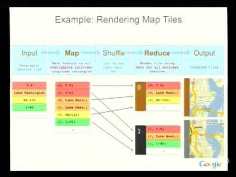
[45:11](https://www.youtube.com/watch?v=modXC5IWTJI&t=2711s) Concrete MapReduce Example: Rendering Google Maps Tiles
Dean illustrates MapReduce using a real-world production example from the Google Maps tile rendering pipeline. The goal is to take a global catalog of raw geographic features (such as roads and bodies of water) and render rasterized map image tiles (e.g., JPEG files) at fixed geographic resolutions. Each output tile across the globe is assigned a distinct numeric identifier (e.g., tile `0`, tile `1`).
Using Seattle geography as an example:
1. **The Map Function**: Receives individual geographic features and determines every tile boundary the feature intersects. If a feature spans multiple boundaries, it emits duplicate records tagged with each respective tile key.
- **Interstate 5 (I-5)**: Crosses both regions; emits key-value pairs for tile `0` and tile `1`.
- **Lake Washington**: Runs north-south across both boundaries; emits records for tile `0` and tile `1`.
- **SR 520 Floating Bridge**: Sits solely in the northern region; emits a record only for tile `0`.
- **Interstate 90 (I-90)**: Sits exclusively in the southern region; emits a record only for tile `1`.
2. **The Shuffle Phase**: The internal framework intercepts intermediate outputs across all workers, sorting and grouping all extracted geometry records by their numeric tile key.
3. **The Reduce Function**: Invoked per unique tile ID, receiving an aggregated list of every intersecting road, bridge, and lake for that bounding box. The user-provided reduce code invokes graphics routines, renders the vector features directly into a raster JPEG image, and writes the tile to persistent storage.
- **Input**: Geographic vector features (roads, waterways, bridges).
- **Map logic**: Geometric intersection test; emits `(tile_id, feature_data)`.
- **Shuffle**: Grouping of all vector data targeting the same spatial tile ID.
- **Reduce logic**: Image rasterization engine outputting final JPEG map tiles.
[47:45](https://www.youtube.com/watch?v=modXC5IWTJI&t=2865s) Runtime Mechanics: Master Coordination and Fine-Grained Tasks
The MapReduce execution framework coordinates work through a centralized master and a fleet of worker processes. A job begins by partitioning input files on the distributed file system into discrete split chunks. The master locates idle worker machines, assigns them map tasks, and tracks execution status. Workers parse their assigned input splits, execute the user's `Map` function, and write intermediate key-value pairs to local disks (or memory buffers). Once mapped data is partitioned—guided by an optional user-defined partitioning function that assigns keys to reduce buckets—idle workers are assigned reduce tasks to pull, sort, and process the clustered key values.
Dean emphasizes that performance at Google's scale is dictated by network bandwidth, disk I/O scheduling, and shuffle efficiency, rather than pure CPU or memory speeds. To ensure rapid fault tolerance, MapReduce employs fine task granularity: workers are assigned 10 to 20 small tasks over a job's lifespan rather than a single monolithic task. If a node fails, its remaining or lost tasks can be distributed concurrently across 20 distinct machines, enabling recovery within seconds while keeping cross-rack network pipelines saturated.
- **Master role**: Splits input data, assigns tasks to idle workers, and handles rescheduling on failure.
- **Storage flow**: Map output writes to local node disks; reduce output writes back to the distributed file system (GFS).
- **Bottlenecks**: Large jobs are bounded by bisection network bandwidth and disk I/O during the shuffle, not CPU/DRAM.
- **Fine-grained scheduling**: Assigning 10–20 small tasks per worker facilitates rapid parallel recovery when individual nodes drop offline.
[50:23](https://www.youtube.com/watch?v=modXC5IWTJI&t=3023s) Pipelining, Fault Tolerance, and Backup Tasks in MapReduce
Jeffrey Dean walks through the finer execution details of MapReduce, illustrating how pipelining and dynamic load balancing keep worker machines maximally utilized. In a setup with multiple workers, the first two are assigned to map tasks—one taking map task 1, finishing rapidly, and immediately picking up map task 3, while the other tackles map task 2, which runs longer. Dean emphasizes that reducers do not sit idle waiting for all map jobs to complete: “So you're actually shuffling in parallel with running other map task computations.” As soon as an individual map task finishes, the assigned reduce workers immediately start pulling its output over the network. Breaking work into finer-grained tasks provides better dynamic load balancing and makes the system resilient to hardware failures, because recovering from a dead machine requires only re-executing its assigned chunks and updating metadata on which node holds the newest outputs.
```mermaid
flowchart TD
accTitle: MapReduce Pipelining and Shuffle Architecture
accDescr: Diagram illustrating concurrent map task execution overlapping with network shuffling into reduce workers.
Dean shares an anecdote demonstrating the framework's fault tolerance during early development. The engineering team suffered crossed signals with data center operations personnel who were rewiring network racks while a massive, experimental MapReduce job was running. Operations continually disconnected rack after rack:
> “...it turns out they were rewiring the network in the data center we were running our large MapReduce on and so they kept unplugging rack after rack of machines rewiring it you know we'd lose 80 machines and like oh well I wonder what's going on and the MapReduce framework would recover and then they'd unplug the next rack and we lose another 80 machines it's quite painful uh but we didn't really know what was going on at the time and it took a little longer than we thought, but we actually handled this and only discovered this after the fact, which is kind of cool.”
Dean then outlines two critical framework optimizations:
- **Backup tasks for stragglers**: When slow workers lag due to extraneous issues (such as local network congestion or concurrent competing jobs) rather than data anomalies, the framework spawns duplicate backup copies near the tail end of the map or reduce phase. Dean notes, “And so we actually run multiple copies of map task seven and whichever one finishes first wins.” This dramatically compresses total job latency.
- **Locality optimization**: Scheduling integrates with the Google File System (GFS) by querying chunk replicas and assigning map tasks directly to the machine holding the physical disk blocks, or at minimum to a node within the same rack.
[53:18](https://www.youtube.com/watch?v=modXC5IWTJI&t=3198s) MapReduce Scale and Introducing Spanner
Reviewing the historical growth of MapReduce internally, Dean highlights its staggering operational throughput. By 2010, Google's MapReduce infrastructure processes nearly an exabyte of data every month across roughly 4 million jobs, a dramatic leap from August 2004 when the monthly workload stood at approximately three terabytes (with Dean and an audience member joking back and forth over petabyte versus exabyte figures: “Uh 946,000 terabytes. Yeah, that's a petabyte. No, nearly an exabyte. Yes.”).
Dean then transitions to a project he is actively co-developing with seven or eight colleagues: Spanner. Unlike prior systems where independent instances were deployed in individual data centers, Spanner is engineered as a unified global infrastructure instance spanning multiple data centers worldwide.
```mermaid
flowchart LR
accTitle: Global Data Access in Spanner versus Disconnected Cells
accDescr: Shows Spanner's single global namespace contrasting with siloed per-datacenter GFS clusters.
subgraph SpannerModel["Spanner Global Namespace"]
GlobalNS["Single Global Namespace<br>Consistent across all Zones"]
ZoneEU["Zone: Europe (2 Replicas)"]
ZoneUS["Zone: US (1 Replica)"]
GlobalNS --> ZoneEU
GlobalNS --> ZoneUS
ClientNew["Client Application"] -->|"Reads uniform path"| GlobalNS
end
```
Dean describes the core motivations and high-level architectural goals of Spanner:
- **Single global namespace**: Eliminates fragile coupling where moving data invalidates resource identifiers. Previously, if the Calendar team relocated data between GFS cells, paths changed and external consumers had to manually ask where the data had moved.
- **Automated cross-datacenter migration**: Replaces labor-intensive, manual coordination with automated data movement and dynamic re-replication across facilities.
- **Consistency across partitions**: Supports a blend of strong and weakly consistent operations globally. Zones are built to operate semi-autonomously, continuing local load balancing and queries during network cuts and reconciling to a consistent view once severed links recover.
- **Declarative policy specification**: Clients declare abstract operational constraints rather than explicit machine locations, expressing intents like wanting three total replicas with two in Europe and one in the United States.
[56:30](https://www.youtube.com/watch?v=modXC5IWTJI&t=3390s) Architectural Lessons: Decoupling and Back-of-the-Envelope Design
Turning to general design experiences and patterns, Dean stresses the necessity of decomposing large, complex software architectures into decoupled subsystems. At Google's scale, distributed RPC services establish clean interfaces that allow autonomous feature velocity. Dean explains: “small teams can work independently of other ones by carefully defining these interfaces and services.” For instance, an engineering group updating the spelling correction engine can deploy revisions at their own cadence without blocking the advertising system or other upstream consumers. Dean notes that every web query hitting Google.com interacts with “200 separate services. Probably more than 200. Who can keep track?” This interface segregation was instrumental in enabling Google to expand from two or three development offices to 30 worldwide within three to four years.
Dean emphasizes that evaluating designs before writing code requires quantitative back-of-the-envelope estimation. Engineers must calculate performance profiles beforehand rather than implementing and benchmarking three failed prototypes to discover poor architectures. Referencing his widely circulated cheat sheet of fundamental latencies, Dean stresses key physical realities:
- Cross-datacenter round-trips are constrained by physical distance and fiber optics (prompting an audience member to marvel that a transatlantic round-trip to the Netherlands represents a significant fraction of the speed of light).
- Memory remains orders of magnitude faster than rotational disk seeks, which should be avoided whenever possible.
- “compress a kilobyte with cheap compression algorithm... often you can get a factor of two compression with a very lightweight compression algorithm and save yourself actually quite a bit of network bandwidth.”
Dean sets up a concrete calculation exercise to demonstrate these principles in practice: estimating the latency required to generate an image search results page displaying 30 thumbnails under different architectural strategies.
[01:00:41](https://www.youtube.com/watch?v=modXC5IWTJI&t=3641s) Back-of-the-Envelope Calculations and System Design
Dean continues walking through an architectural calculation example involving disk reads. In the first design, fetching an image involves performing a disk seek, reading a quarter-megabyte image, and then moving sequentially to the next image, taking roughly half a second in total. In contrast, issuing reads in parallel across a sufficient number of disks cuts retrieval time down to around 20 milliseconds. While real-world variance across many disks means some will naturally run slower than others, parallel reads remain significantly faster than the sequential approach.
Dean emphasizes that performing back-of-the-envelope calculations allows an engineer to quickly explore numerous design variations: whether it makes sense to cache individual thumbnails, bundle entire sets of thumbnails into a single cache entry, or precompute thumbnails entirely. He argues that engineers must run these numbers continuously during the design process, stressing that designers must also understand the baseline performance of the underlying primitives: “If you don't know, you know, roughly how long it takes to do a write into your cache system, uh, then by cache, I mean like a disk based cache, higher level software system, then you really can't tell if it's a good idea to cache things or not.”
- **Sequential reads vs. parallel reads**: Sequential reads take roughly 500 ms due to cumulative disk seeks and 250 KB data reads; parallel reads across separate disks cut this down to ~20 ms (plus variance).
- **Evaluating caching trade-offs**: Calculating whether to store individual image thumbnails, group sets of thumbnails together, or precalculate them ahead of time.
- **Baseline awareness**: Designing a caching layer requires knowing the read/write latency of lower-level storage layers to evaluate if caching is actually beneficial.
---
[01:02:08](https://www.youtube.com/watch?v=modXC5IWTJI&t=3728s) Building Shared Infrastructure: Needs, Feature Creep, and Dogfooding
When creating shared software infrastructure for multiple teams, clients will inevitably request an overwhelming assortment of features. Dean points out that the crucial skill is finding the common denominator among those requests. If users ask for eight different features, six are usually shared across groups, and implementing those six will satisfy most needs. While an engineering team can stretch to accommodate a seventh, attempting to build all eight invariably overburdens the system: “Uh, but if you try to do all eight, it's really going to probably work result in a worse system for everyone because the system will get much more complicated because that eighth feature just drove you over the edge of complexity in some way.” An audience member asks about focusing on “what they need instead of what they want,” to which Dean agrees that engineers must translate requests, often finding that providing one fundamental feature eliminates the user's perceived need for another.
Dean warns strongly against building infrastructure merely because it is intellectually enjoyable or designing for hypothetical users with speculative requirements. The most effective safeguard against overengineering is dogfooding—building an application on top of the infrastructure while simultaneously implementing the infrastructure itself. This tight feedback loop allows developers to make rapid, pragmatic decisions about whether a specific capability belongs in the shared infrastructure layer or directly inside the application. If dogfooding is not possible, infrastructure teams should sit directly next to their users to maintain an equally fast feedback cycle.
- **The feature-limit rule**: Build the common 6 out of 8 requested features; stretching to 7 may work, but chasing all 8 introduces complexity that degrades the system for everyone.
- **Wants vs. needs**: Translating client requests into underlying core abstractions often removes the need for niche, complex feature requests.
- **Avoiding hypothetical traps**: Build to address concrete, current needs rather than imagining elaborate edge cases that nobody has asked for today.
- **Close proximity iteration**: Developing applications directly on top of the underlying infrastructure provides instant feedback on API ergonomics and usability.
---
[01:04:37](https://www.youtube.com/watch?v=modXC5IWTJI&t=3877s) Designing for Growth and the Power of Centralized Control
Engineering for growth requires anticipating which parameters will scale over time, though Dean notes that building a system to scale infinitely from day one is a mistake. When system metrics change by two orders of magnitude, the fundamental architecture typically needs to change as well. In Google's search infrastructure, the original disk-based index evolved well up to a point, but once query traffic increased by a factor of 100x, it became necessary to transition to an entirely in-memory index. As Dean summarizes: “Um and so when you have parameters that change by two orders of magnitude that probably means the original design is not going to be the right one at that much larger scale.”
```mermaid
flowchart TD
accTitle: Centralized Master Architecture
accDescr: A centralized master coordinates worker nodes while staying off the high-frequency data path.
Master -->|"infrequent control / tasks"| W1
Master -->|"infrequent control / tasks"| W2
Master -->|"infrequent control / tasks"| W3
W1 <-->|"direct data transfer"| W2
W2 <-->|"direct data transfer"| W3
```
Dean also addresses the architectural trade-off between fully decentralized peer-to-peer state and centralized coordination. While distributed systems engineers are often tempted to avoid single points of coordination, centralized masters have proven remarkably effective in systems like the Google File System (GFS) for metadata, Bigtable for load balancing, and MapReduce for task scheduling. Keeping the master off the high-frequency data path prevents it from becoming a bottleneck, enabling a single coordinator to manage fleets of 1,000 to 10,000 machines cleanly while simplifying system monitoring and state reasoning.
- **The 100x redesign threshold**: A system architecture rarely survives a two-orders-of-magnitude shift; scaling 100x typically calls for a completely different design rather than incremental patches.
- **Centralized master utility**: GFS, Bigtable, and MapReduce all utilize centralized coordinators to maintain state and handle machine oversight.
- **Staying off the critical path**: Central masters scale to thousands of workers provided they are kept out of frequent, fine-grained data-plane operations.
- **Hot standbys**: Running a hot standby allows rapid recovery if the primary master fails.
---
[01:07:13](https://www.youtube.com/watch?v=modXC5IWTJI&t=4033s) Tree Distribution, Tail-Latency Backups, and Fine-Grained Work Units
When broadcasting queries to large clusters, directing hundreds of leaf nodes to respond to a single root node causes severe network bottlenecks. This high fan-in saturates the root's network interface and CPU, triggering TCP packet drops and retransmissions that introduce high latency tails. Introducing an intermediate tree structure solves this problem. Parent nodes send requests to assigned subsets of leaves and aggregate the responses, dramatically reducing the root's CPU burden and network load. In Google's search system, leaves produce their top 10 or 15 results, and the intermediate parent selects the best 20 or 30 results from its 30 leaf nodes before sending them upstream. Tree topologies also align cleanly with rack boundaries, keeping high-volume communication within rack switches where bandwidth is plentiful.
```mermaid
flowchart TD
accTitle: Tree-Structured Request Fanout and Aggregation
accDescr: A root node fans out requests through rack-level parent aggregators to leaf nodes.
Root -->|"query fanout"| P1
Root -->|"query fanout"| P2
P1 -->|"filtered top 20-30"| Root
P2 -->|"filtered top 20-30"| Root
```
To combat tail latency, Dean describes issuing backup requests to replicas near the end of an operation. While MapReduce launches speculative backup tasks over horizons of many seconds, search serving applies this strategy at millisecond granularity: “And so if you have multiple replicas towards the end of sending it out to all thousand leaves, if you've heard back from 995 and you have replicas for the other five, why not send, you know, five extra requests to the replicas and see which ones respond first?” Finally, Dean highlights the importance of splitting machine workloads into multiple smaller units; assigning monolithic tasks to single machines makes recovery painfully slow when hardware fails, as replacement nodes are forced to reload massive blocks of state.
- **Mitigating wide fan-in**: Hierarchical trees prevent TCP packet drops, buffer overruns, and root CPU exhaustion caused by hundreds of leaves replying at once.
- **Parent filtering**: Intermediate parent nodes aggregate responses from ~30 leaves, filtering hundreds of candidate documents down to the top 20–30 before forwarding them to the root.
- **Locality-aware aggregation**: Mapping parent nodes to specific server racks optimizes for intra-rack bandwidth where bisection bandwidth across the datacenter is constrained.
- **Millisecond-level backup requests**: Dispatching duplicate requests for the slowest 5 out of 1,000 leaf queries curbs long-tail latency.
- **Granular work units**: Breaking responsibilities into small units ensures fast failover, preventing recovery nodes from having to rebuild massive monolithic states.
[01:09:49](https://www.youtube.com/watch?v=modXC5IWTJI&t=4189s) Granular Work Chunks and Elastic Systems Under Overload
Jeffrey Dean concludes his discussion of system architecture patterns by emphasizing the danger of monolithic work units. When work is treated as a single monolithic block, systems become exceptionally brittle. It creates severe inflexibility for load balancing: if a particular machine becomes overloaded because its assigned chunk is slightly more computationally expensive, an operator has virtually no recourse because moving the monolithic task to another machine will simply make that second machine slow as well. In contrast, breaking work into finer grains—giving 10, 20, or 100 small chunks to a single machine—delivers dramatic advantages for both recovery and load balancing. Dean points out that “if this machine dies nine other machines can each pick up one of these chunks and recover uh in one ninth the time the monolithic one could and it also gives you load balancing.” Shedding a single chunk instantly frees up capacity and brings an overloaded server back to a healthy state, an architectural design pattern pervasive across Google's infrastructure.
Dean then highlights the necessity of designing elastic systems. Predicting peak load is inherently difficult because traffic fluctuates across the day and can surge abruptly due to denial-of-service (DoS) attacks or query floods. While an elastic architecture should ideally scale down capacity at night when traffic dips and ramp it back up during daytime peaks, elastic scaling takes time to provision. Systems must therefore remain resilient when hit by sudden, unexpected overload, maintaining reasonable behavior even under double the expected query volume. Rather than failing completely, systems should gracefully degrade:
- In Google Web Search, the engine can truncate the tail of the corpus, querying only the top few billion documents instead of the full index, trading a small amount of quality for responsiveness since Dean stresses that “your quality will suffer a little bit but you're overloaded and it's better to return responses than not.”
- Non-essential auxiliary services can be dropped entirely under load, such as bypassing spelling correction suggestions if the spelling backend begins to experience latency spikes.
- Load balancing mechanisms can become progressively more aggressive as server imbalances grow more severe, redistributing work dynamically to absorb the shock.
```mermaid
flowchart TD
accTitle: Elastic Overload Handling Architecture
accDescr: Flow diagram showing graceful degradation and fine-grained chunk recovery under heavy server load.
subgraph S1["Incoming Query Spike"]
Traffic["Unexpected Traffic Spike (2x Normal Load)"]
end
subgraph S2["Graceful Degradation"]
Traffic --> Search["Web Search Processing"]
Search -->|"Shed Tail Load"| Tail["Truncate Deep Index (Search Top Billions Only)"]
Search -->|"Drop Auxiliaries"| Spell["Bypass Latent Spell Checker"]
end
subgraph S3["Fine-Grained Elastic Rebalancing"]
Traffic --> Tasks["Decompose into Fine Chunks (10-100 Per Machine)"]
Tasks --> Recover["Fast Multi-Machine Recovery (1/9th Time)"]
Tasks --> Balance["Aggressive Load Redistribution"]
end
```
[01:12:08](https://www.youtube.com/watch?v=modXC5IWTJI&t=4328s) Final Thoughts and Q&A: Borg Scheduling and Data Center Networking
Dean wraps up the formal lecture by skipping an unneeded slide to reflect on the modern computing landscape. He observes that computer science has entered an extraordinarily exciting era defined by the convergence of massive computational power aggregated in single locations, massive datasets encompassing large fractions of human knowledge online, and a proliferating ecosystem of increasingly powerful client devices interacting with data center services. Directing attendees to research papers published at `labs.google.com/papers`, he opens the floor to audience questions.
The initial question addresses how applications specify resource requirements when deploying to Google data centers—specifically whether they request fungible resources or more complex allocations. Dean explains that at Google's scheduling level (Borg), developers request a specific count of tasks, each defined by an explicit multidimensional vector of required resources:
- CPU cores (e.g., requesting two cores per task).
- Memory limits (in megabytes or gigabytes).
- Disk space and network bandwidth.
The scheduling infrastructure then solves a massive multidimensional bin-packing problem to place those tasks onto physical machines, with higher-level deployment abstractions layered on top to shield developers from manual low-level specifications. An attendee jokingly asks if the scheduling is "nerd-centric," to which Dean laughs, clarifies that the question was "node-centric," and humorously replies, “Yeah, well that too.” Addressing how software interacts with physical network infrastructure, Dean notes that datacenter networks have evolved continuously to supply higher bisection bandwidth, expanded capacity, and lower latency. Although software and network infrastructure evolve in parallel tracks, the teams maintain active coordination to project network capabilities a year in advance and design systems to exploit them.
[01:15:02](https://www.youtube.com/watch?v=modXC5IWTJI&t=4502s) Future Infrastructure Challenges: Spanner, Storage Scaling, and Energy
When asked what big infrastructure challenges keep him awake at night, Dean identifies cross-data-center service orchestration as a primary bottleneck. Historically, Google's tools evolved around individual data centers, forcing teams to rely on a patchwork of disconnected utilities—such as separate scripts for file transfers and fragmented job-monitoring consoles. Dean explains that the development of Spanner was conceived specifically to address this pain point: “I think you know one of them which is uh Spanner is partly a response to is that it's very hard when you're operating a service that needs to run in multiple data centers because a lot of the infrastructure we've built to this point has been very data center ccentric.” Unifying this multi-datacenter operational environment remains essential to tame software complexity.
Subsequent audience questions explore physical scaling limits, data volumes, power consumption, and specialized algorithms:
- **Web Corpus Growth vs. Storage Hardware:** An audience member asks whether the expanding web will outstrip hardware storage advancements. Dean distinguishes textual content from rich media: the textual web is growing slower than storage hardware density, allowing a substantial portion of all online text to reside on a few hundred hard drives within a single server rack. However, video content generated by ubiquitous high-definition devices creates immense bandwidth and storage burdens. Dean quips: “You will not have all the world's video in your pocket anytime soon. Let me put it that way.”
- **Datacenter Power and Energy Proportionality:** Asked how Google will pay its electricity bills in 20 years, Dean jokes, “probably through ads,” before addressing the technical realities of data center efficiency. He notes that modern machines lack energy proportionality: a server utilizing only 50% of its CPU capacity typically consumes 70% to 80% of its peak power. Long-term research must target energy-proportional hardware, low-power CPU architectures, and aggressive software idling to curb escalating power costs.
- **Computing PageRank on MapReduce:** A member of the audience asks how Google optimizes PageRank computations and why few MapReduce optimizations have been published. Dean clarifies that while PageRank can be computed on MapReduce by iteratively reading the link graph, propagating weights, and emitting outputs across each stage, MapReduce is not inherently optimal for iterative graph processing. While MapReduce is fantastic for rapid prototyping without premature optimization, Dean notes that when computing at the scale of thousands of machines, engineering teams justify the investment to construct bespoke, specialized processing systems rather than forcing graph workloads into a pure MapReduce paradigm.
[01:19:28](https://www.youtube.com/watch?v=modXC5IWTJI&t=4768s) MapReduce Chains and Intermediate Storage
An audience member asks Jeffrey Dean whether Google uses design patterns that resemble chained MapReduce workflows. Dean confirms that this is indeed standard practice, explaining that complex algorithms are frequently structured as a linked sequence of distinct MapReduce jobs. In this setup, the output generated by the reduce phase of one stage feeds directly into the subsequent map stage of the next job, breaking down a large multi-step computation into discrete, manageable pieces.
When asked whether the intermediate stages write out and read back data between phases, Dean elaborates on storage trade-offs. Because the intermediate data generated across an algorithmic chain is transient and the entire computation can be rerun from scratch if a node or disk fails, Google can opt to write intermediate outputs to a cheaper, less durable storage tier rather than fully redundant storage. As Jeffrey Dean explains:
> “Um but a pretty common pattern is to have a whole change sequence of map produces that each do some part of a larger algorithm in a sequence of steps.”
- MapReduce chains execute multi-step algorithms sequentially, passing intermediate datasets from one job's reducers into the next job's mappers.
- Intermediate pipeline data is often written to cheaper storage tiers because it is fully reproducible if a failure occurs.
---
[01:20:13](https://www.youtube.com/watch?v=modXC5IWTJI&t=4813s) The Infrastructure Impact of Google Instant
The discussion turns to Google Instant and how its real-time, search-as-you-type functionality affects the underlying infrastructure. Dean explains that Google Instant operates continuously in the background while a user types: it predicts the full query from just a few initial keystrokes and proactively prefetches search results before the user finishes typing or hits Enter.
Dean emphasizes that supporting Google Instant did not require a fundamental re-architecture of Google's underlying web search infrastructure; rather, it is primarily a capacity and load-management challenge. To keep the serving system resilient under heavy load, predictive requests are explicitly marked so the system knows their priority. Furthermore, because predicted queries correspond to popular historical searches, they benefit significantly from caching. As Jeffrey Dean points out:
> “One of the things we do is uh when I mentioned making your system resilient to overload, those requests come tagged with a bit that says they're a predictive prefetch, not something the user actually pressed uh enter on.”
```mermaid
flowchart LR
accTitle: Google Instant Request Flow
accDescr: Pipeline showing user keystroke generation, query prediction, conditional dropping under overload, and cached result retrieval.
subgraph UserInteraction["User Interaction"]
A["User Keystrokes"] --> B["Predictive Query Engine"]
end
subgraph RequestHandling["Request Classification"]
B --> C{"System Overloaded?"}
C -- "Yes" --> D["Drop Request"]
C -- "No" --> E["Tagged Prefetch Request<br/>(Predictive Bit Set)"]
end
subgraph Serving["Search Serving"]
E --> F["Result Cache / Search Backend"]
F --> G["Prefetched SERP Returned"]
end
```
- Google Instant predicts queries and prefetches search results dynamically as the user types characters into the search bar.
- Requests carry a dedicated metadata bit designating them as speculative prefetches rather than explicit user submissions.
- When search clusters experience overload, predictive prefetch requests can be safely discarded without degrading explicit user interactions.
- Predictive queries demonstrate high cache hit rates because predictions naturally align with queries commonly issued by users in the past.
---
[01:21:22](https://www.youtube.com/watch?v=modXC5IWTJI&t=4882s) Distributed Transactions: From Bigtable Regrets to Spanner
For the final question of the talk, an audience member asks about Google’s experience with distributed transactions within a single data center. Dean candidly reflects on how Google's infrastructure strategy historically avoided general distributed transactions. When designing Bigtable, the team intentionally restricted transactional guarantees to single-row updates, leaving distributed multi-row or multi-table transactions out of the core system.
Dean admits that omitting distributed transactions from early systems was a strategic miscalculation. Because product teams genuinely required multi-entity transactions, developers were forced to implement their own ad hoc coordination protocols—frequently making mistakes along the way. Even inside Bigtable itself, engineers hand-rolled custom transactional protocols to support certain subtle internal features. To correct this systemic problem, Google incorporated native distributed transactions into Spanner so that all developers have access to a robust, shared implementation. As Jeffrey Dean reflects:
> “Um, in retrospect, I think that was a mistake. Uh, we probably should have added them in because what ended up happening is a lot of people did want distributed transactions and so they handrolled their own protocols.”
- Bigtable originally provided atomicity and isolation exclusively at the single-row level.
- Omitting cross-row and cross-machine transactions forced product teams to invent bespoke transactional protocols, which were prone to subtle correctness bugs.
- Bigtable's internal implementation had to rely on custom, hand-rolled protocols for some of its own advanced features.
- Spanner directly addresses these historical shortcomings by providing native distributed transactions across the entire infrastructure layer.
## Notable quotes
> [01:04:37](https://www.youtube.com/watch?v=modXC5IWTJI&t=3877s) when you have parameters that change by two orders of magnitude that probably means the original design is not going to be the right one at that much larger scale. — Jeffrey Dean
> [56:30](https://www.youtube.com/watch?v=modXC5IWTJI&t=3390s) small teams can work independently of other ones by carefully defining these interfaces and services. — Jeffrey Dean
> [01:09:49](https://www.youtube.com/watch?v=modXC5IWTJI&t=4189s) if this machine dies nine other machines can each pick up one of these chunks and recover uh in one ninth the time the monolithic one could and it also gives you load balancing. — Jeffrey Dean
> [01:09:49](https://www.youtube.com/watch?v=modXC5IWTJI&t=4189s) your quality will suffer a little bit but you're overloaded and it's better to return responses than not. — Jeffrey Dean
> [05:37](https://www.youtube.com/watch?v=modXC5IWTJI&t=337s) From a performance standpoint in a search engine, the cost is dominated by the index serving portion. The doc serving portion really doesn't matter at all, which is why you won't hear me talk about it too much. — Jeff Dean
> [01:02:08](https://www.youtube.com/watch?v=modXC5IWTJI&t=3728s) Uh, but if you try to do all eight, it's really going to probably work result in a worse system for everyone because the system will get much more complicated because that eighth feature just drove you over the edge of complexity in some way. — Jeffrey Dean
> [01:21:22](https://www.youtube.com/watch?v=modXC5IWTJI&t=4882s) Um, in retrospect, I think that was a mistake. Uh, we probably should have added them in because what ended up happening is a lot of people did want distributed transactions and so they handrolled their own protocols. — Jeffrey Dean
> [01:07:13](https://www.youtube.com/watch?v=modXC5IWTJI&t=4033s) And so if you have multiple replicas towards the end of sending it out to all thousand leaves, if you've heard back from 995 and you have replicas for the other five, why not send, you know, five extra requests to the replicas and see which ones respond first? — Jeffrey Dean
## Mentioned
Bigtable, Borg, Chubby, CNN.com, Digital Equipment Corporation, Google, Google File System (GFS), Google Instant, Google Maps, Google Web Server (GWS), IBM, Jeff Dean, Larry Page, Linux, MapReduce, PageRank, Protocol Buffers, Sanjay Ghemawat, Sergey Brin, Spanner, Stanford University, Sun Microsystems, Universal Search, University of Washington, Western Research Laboratory, Yahoo
## Video description
(November 10, 2010) Speaker Jeffrey Dean describes some of his experiences at Google and the types of technology being used today. He talks about how their technology has evolved over time and how their technological infrastructure has allowed them to be so successful.
Stanford University:
http://www.stanford.edu/
School of Engineering:
http://soe.stanford.edu/
Stanford Center for Professional Development:
http://scpd.stanford.edu/
Stanford University Channel on YouTube:
http://www.youtube.com/stanford
谷歌软件系统构建与经验教训
Jeff Dean回顾了谷歌核心搜索与分布式基础设施11年的演进历程,详细阐述了公司在查询量、文档量和计算能力增长1000倍的过程中,如何经历约七次完整的系统重写来实现规模扩展。他解释了关键的架构转折点,包括从受限于磁盘的软木板PC集群过渡到高吞吐内存搜索索引,以及将临时的分布式流水线抽象为GFS、MapReduce、Bigtable和Spanner等基础系统。在整个演讲中,Dean强调了实用的分布式设计模式,例如将工作负载拆分为细粒度分块、通过备份任务缓解尾部延迟,以及在实现前进行粗略的延迟估算。最后,他总结了来之不易的运维经验,探讨了多数据中心协同面临的挑战,以及为何在Bigtable中舍弃分布式事务被证明是一个设计遗憾,并最终在Spanner中得以修正。
在1999年至2010年间,谷歌的索引规模和查询量各增长了约1000倍,在保持稳定的面向用户界面的同时,需要对搜索架构进行大约七次彻底的从头重写。 (2:41)
2001年,谷歌从基于机械磁盘的索引检索转向完全基于内存的索引架构,消除了磁盘寻道瓶颈并大幅降低了尾部延迟。 (19:05)
到2010年,MapReduce每月通过400万个作业处理近1 EB(约946,000 TB)的数据,从而推动了Spanner的开发,以提供跨数据中心的全局分布式命名空间。 (53:18)
Jeff Dean承认,Bigtable中舍弃多行分布式事务是一个历史性错误,该设计迫使应用团队自行实现充满错误的临时协议,最终促成了Spanner对原生事务的支持。 (81:22)
Reading summary
In a Stanford colloquium, Google Fellow Jeff Dean outlines how Google evolved its computational systems from fragile commodity PC clusters into resilient, planetary-scale distributed infrastructure, emphasizing that major orders-of-magnitude growth require completely rethinking architectural primitives.
Commodity Hardware and In-Memory Index Evolution (8:28)
Google initially relied on cheap desktop components, such as custom trays packing four PCs on corkboard insulation with shared power supplies, to maximize compute per dollar. However, early consumer hardware lacked ECC memory and parity, forcing software engineers to write custom formats with checksums and synchronization markers to survive corrupted state during batch sorting. Between 1999 and 2001, index size expanded 20x and traffic doubled overnight following the July 2000 Yahoo deal, hitting the physical limits of disk seeks on phrase queries like 'circle of life.' In 2001, aggregate cluster RAM grew large enough for Google to move its inverted index entirely into memory.
Mitigating Latency Tails and Cascading Failures (20:28)
Transitioning to an in-memory index required fanning out individual queries across thousands of backend machines, which exacerbated tail latencies. Well-intentioned operational decisions, such as staggering five-minute cron jobs randomly across hosts, actually increased latency variance across large clusters. To mitigate cascading failures from 'queries of death'—malformed requests that could crash an entire tier—Google implemented canary requests that probe a single host before broadcasting to the rest of the cluster. In 2004, the architecture was redesigned with unified leaf servers combining index retrieval and document summary generation, organized into multi-level distribution trees with intermediate aggregators.
Abstracting Distributed Processing with MapReduce (41:23)
As crawling expanded to datasets such as 20 billion web pages (roughly 400 terabytes), running monolithic sequential processing became impossible, taking months instead of hours on a thousand machines. In 2003, Jeffrey Dean and Sanjay Ghemawat extracted common patterns from bespoke indexing pipelines into MapReduce. The system shielded developers from network handoffs, task distribution, and fault tolerance by exposing simple Map and Reduce functions. MapReduce relies on fine-grained task scheduling (10 to 20 tasks per worker) and pipelined shuffling to dynamically balance loads and quickly reschedule failed chunks onto surviving workers. By 2010, internal MapReduce infrastructure was processing nearly an exabyte monthly across roughly 4 million jobs.
Core Engineering Patterns and Architectural Lessons (56:30)
Dean underscores that when operational parameters shift by two orders of magnitude, system architectures must be redesigned. System designers should rely on back-of-the-envelope calculations using fundamental latency profiles—such as memory versus rotational disk speeds—to discard unworkable ideas before writing code. To keep infrastructure stable, Dean recommends centralizing master state coordination while keeping data transfers direct between workers, dogfooding infrastructure applications to prevent feature creep, and breaking workloads into fine chunks to enable elastic shedding and fast recovery during unexpected traffic surges.
Global Data Centers and the Transaction Miscalculation (53:18)
As systems expanded globally, managing independent per-data-center storage cells became an operational bottleneck, motivating the development of Spanner's unified global namespace. Dean candidly reflects that omitting multi-row distributed transactions from Bigtable was a strategic mistake: developers across product teams genuinely needed transactional guarantees and ended up writing error-prone, ad hoc protocols. Spanner was designed to provide native, robust distributed transactions globally to eliminate this systemic issue across the organization.
Dean emphasizes that managing cross-datacenter orchestration remains an ongoing infrastructure challenge. While storage capacity comfortably scales ahead of the growth of online text, explosive rich media like high-definition video continues to exert severe strain on global network bandwidth and storage.
精炼阅读摘要
在斯坦福大学的演讲中,Google Fellow Jeff Dean系统阐述了Google在面对数据与流量呈千倍规模扩张时,如何通过软硬件协同、计算范式抽象以及系统解耦等工程原则,构建高吞吐且容错的分布式基础设施。
从廉价硬件到全内存检索架构的演进 (8:28)
Google在发展初期受预算限制,选择使用消费级PC配件拼装服务器(如用软木板绝缘的机架托盘),但无校验内存频繁导致数据在大规模排序时出现静默翻转,迫使工程师在软件层实现校验和与断点重同步机制。1999年至2010年间,网页索引量与每日查询量均增长了约1000倍,2000年与雅虎达成合作更导致流量一夜之间翻倍。早期的磁盘倒排索引在面对如“circle of life”等高频词组查询时,单次请求甚至需要读取高达30GB的数据,机械寻道逐渐成为性能死锁点。
全内存检索的工程陷阱与系统优化 (19:05)
2001年,Google利用集群总体RAM的容量优势全面转向内存索引。然而,内存架构放大了长尾延迟与集群抖动风险:运维此前交错运行的5分钟定时清理脚本反而在大扇出集群中持续引入微卡顿;同时,能导致单机崩溃的“死亡查询”(Query of Death)在广播给上千台机器时可能击垮整个数据中心,促使团队设计了先打向单机的金丝雀请求机制。此外,为优化CPU解码吞吐,系统逐步放宽了磁盘时代的极致压缩策略,转而采用以4个数字为一组、配以1字节前缀头的定长解码方案,通过查表消除分支预测失败,使解码性能提升了约两倍。
计算与存储原语的通用抽象 (37:34)
面对200亿网页、约400TB数据的离线批处理挑战,单机处理需耗时数月,而早期定制化的分布式管道充斥着重复的网络容错与状态同步代码。2003年起,Google相继推出了GFS与MapReduce:GFS通过分离主控元数据与数据块流,高效存储大文件;MapReduce则将提取与聚合逻辑抽象为简单的Map和Reduce接口,将底层的网络洗牌、细粒度任务调度以及应对落后节点的备份任务自动化,使每月处理量在2010年达到近1EB的规模。在跨数据中心协调方面,新系统Spanner被设计用来打破原本按单个数据中心隔离的孤岛模型,提供统一的全局命名空间。
规模化工程原则与事务支持的反思 (56:30)
Dean总结了多项设计经验:任何系统当关键参数跨越两个数量级时,往往需要彻底推翻重构;复杂的单体逻辑应通过清晰的RPC服务拆分为解耦子系统(当时Google搜索一次请求会触达超过200个独立服务);同时,必须依赖粗略的数量级估算(Back-of-the-Envelope Calculation)在编码前验证延迟模型。Dean还坦承,Bigtable最初仅支持单行事务是一个设计失误,导致上层产品团队不得不自行编写极易出错的分布式协调协议,促使团队在Spanner中直接下沉并原生支持分布式事务。
Dean指出,计算机科学已步入由超大规模计算、全人类数字化知识与强大终端汇聚的新时代,而跨数据中心的自动化编排以及海量视频数据带来的存储与能耗挑战,仍是未来分布式系统亟待解决的核心难题。
Source quotes
[64:37] Jeffrey Dean: when you have parameters that change by two orders of magnitude that probably means the original design is not going to be the right one at that much larger scale.
[56:30] Jeffrey Dean: small teams can work independently of other ones by carefully defining these interfaces and services.
[69:49] Jeffrey Dean: if this machine dies nine other machines can each pick up one of these chunks and recover uh in one ninth the time the monolithic one could and it also gives you load balancing.
[69:49] Jeffrey Dean: your quality will suffer a little bit but you're overloaded and it's better to return responses than not.
[5:37] Jeff Dean: From a performance standpoint in a search engine, the cost is dominated by the index serving portion. The doc serving portion really doesn't matter at all, which is why you won't hear me talk about it too much.
[62:08] Jeffrey Dean: Uh, but if you try to do all eight, it's really going to probably work result in a worse system for everyone because the system will get much more complicated because that eighth feature just drove you over the edge of complexity in some way.
[81:22] Jeffrey Dean: Um, in retrospect, I think that was a mistake. Uh, we probably should have added them in because what ended up happening is a lot of people did want distributed transactions and so they handrolled their own protocols.
[67:13] Jeffrey Dean: And so if you have multiple replicas towards the end of sending it out to all thousand leaves, if you've heard back from 995 and you have replicas for the other five, why not send, you know, five extra requests to the replicas and see which ones respond first?
Original transcript
[0:00] [Music]
[0:05] Stanford
[0:23] University.
[0:25] Okay. Can you hear me? Okay. Okay. Um,
[0:28] welcome to I guess this is E380, but
[0:31] it's also been sort of overridden with
[0:33] our distinguished lecture series. Um,
[0:36] today's speaker is Jeff Dean of Google.
[0:38] And um, you know, Jeff, you know, I
[0:41] don't want to use up all his time
[0:43] describing all his accomplishments, but
[0:45] I'll say he did get his degree at
[0:47] University of Washington, but since his
[0:50] adviser was a graduate of here, we can
[0:52] claim him as a grandchild of our
[0:54] institution, and we we certainly do
[0:57] that. Um he he initially landed after
[0:59] his degree at Deck um research lab
[1:02] worked there for a while and then made
[1:04] the smart move to jump over to Google in
[1:06] the early days where he was an
[1:08] instrumental in building a lot of the
[1:09] systems that Google uses to make money
[1:12] basically their search and language
[1:15] translation all all these things and
[1:17] along the way he was involved with some
[1:19] very influential in um pieces of
[1:21] infrastructure including big table map
[1:24] reduce and protocol buffers and so um
[1:27] that introduction, I'll let let Jeff
[1:29] describe them to you. Thank you, Malle.
[1:31] Um, so welcome. Uh, thank you for having
[1:33] me.
[1:35] Uh, I will try to speak louder. Um, so
[1:39] the plan for today is, uh, I'm going to
[1:41] connect my
[1:43] microphone. Um, I'm going to talk about
[1:46] the evolution of various different kinds
[1:48] of systems at Google. One is how our
[1:50] computing hardware has evolved over
[1:52] about the last decade or so. And another
[1:55] thing is about how our core web search
[1:57] and uh retrieval systems have evolved.
[2:00] Uh what we've done in order to scale
[2:02] those systems as traffic and index sizes
[2:04] have grown and so on. I'll talk a little
[2:06] bit about some of the infrastructure
[2:07] software we've built that also underlies
[2:09] a bunch of Google products. uh and then
[2:12] uh the sec the last little bit of the
[2:14] talk I'm going to talk about uh some of
[2:16] the techniques that we've developed to
[2:17] de to build high performance and
[2:19] reliable systems that have kind of
[2:21] cropped up in the process of building
[2:23] some of these systems and sort of
[2:24] general patterns that seem useful uh
[2:26] across a wide variety of kinds of
[2:28] systems. Uh this is joint work with a
[2:30] huge number of people at Google. Um I've
[2:32] worked on all the systems I'm describing
[2:34] but there were many many people involved
[2:36] and I always appreciate my my
[2:38] colleagues. Um
[2:41] so when I started working on web search
[2:44] in 1999 at Google uh these are some
[2:47] metrics that uh I think you can use to
[2:50] uh evaluate different dimensions of a
[2:52] retrieval system. One is how many
[2:54] documents you're indexing and that scale
[2:56] has increased by about a factor of a
[2:58] thousand from 1999 to today. Uh the
[3:01] second thing that is another important
[3:04] dimension is how many queries you have
[3:06] to handle on a given day and that's also
[3:07] grown by a factor of a thousand. I have
[3:09] a quick experiment. How many of you use
[3:11] Google regularly in 1999?
[3:15] Yeah, this may be a biased audience
[3:18] but how about 2002?
[3:22] How about
[3:23] now? Okay. Yeah. Well, so our traffic
[3:25] has grown but I don't see a thousand
[3:27] more hands than I did earlier.
[3:29] Um, another important thing that is
[3:33] uh pretty vital for improving your
[3:35] ranking quality is often you want to
[3:37] keep additional information about around
[3:38] about each document in your index and
[3:41] use that to uh you drive more
[3:43] sophisticated ranking algorithms. And
[3:44] the amount of information we keep in our
[3:46] index today is about three times as much
[3:48] as it was uh then per document. Um, one
[3:52] of the things when I was making this
[3:53] slide that was kind of surprising is
[3:54] that the the metric that's grown the
[3:56] most or improved the most is actually
[3:58] our update latency. In 1999, we were
[4:00] basically updating our index uh once a
[4:02] month if we were lucky and once every
[4:04] couple months if something horrible went
[4:06] wrong. And now we have uh portions of
[4:08] our index we can update within a matter
[4:10] of seconds uh from crawling the page.
[4:12] And so that's a pretty substantial
[4:14] improvement. Uh the other important
[4:16] factor for users is how quickly do you
[4:18] get your responses? uh this is measured
[4:20] at the server side not doesn't include
[4:21] client side network latency but um
[4:24] basically you know we've had about a 5x
[4:25] improvement in there. Um so the
[4:28] difficulty in kind of engineering a
[4:30] retrieval system is in some sense the
[4:32] product of all these things because
[4:33] you're dealing with larger indices.
[4:35] You're trying to handle more queries uh
[4:37] with more information per document and
[4:39] you're trying to update it more often
[4:40] and you're trying to do it faster. Um,
[4:43] now one thing that's really helped us a
[4:44] lot is that we've uh been able to use
[4:47] more machines and faster machines uh
[4:50] since 1999. We've uh upgraded our
[4:52] hardware a bit. Um, and that's given us
[4:54] about a thousandx improvement in sort of
[4:56] computational oomph.
[4:59] Um, the other kind of cool thing about
[5:01] working on search is that uh a lot of
[5:03] the stuff kind of happens behind the
[5:05] scenes and we don't necessarily change
[5:07] the user interface every time we change
[5:08] kind of how the guts of our search
[5:10] system work. And so over the last 11
[5:12] years, we've rolled out about seven very
[5:15] significant revisions to how our search
[5:17] system
[5:18] works. And often these have been rolled
[5:20] out without users really realizing we've
[5:22] made major fundamental changes
[5:24] underneath the covers. Other than
[5:26] perhaps, you know, seeing a larger index
[5:28] or responses uh faster, things like
[5:31] that, the UI kind of looks the
[5:34] same. Uh okay, so I will start at the
[5:37] beginning.
[5:39] Uh so as you obviously know Larry and
[5:42] Sergey were grad students here and were
[5:44] doing research on how to build sort of
[5:46] uh search engines for web uh pages and
[5:49] using the link structure of the web in
[5:51] order to do interesting ranking
[5:52] experiments. Uh, apparently their
[5:54] advisers were very mean and would not
[5:56] buy them enough computers. And so they
[5:58] apparently survived by um going down to
[6:01] the loading dock and uh volunteering to
[6:03] set up other other research groups
[6:05] machines and then living off the float
[6:06] for a while while they would actually
[6:07] use the machines for a little while. Uh,
[6:09] one problem with this approach is um you
[6:11] end up with kind of a heterogeneous mix
[6:13] of suns and IBMs and all kinds of crazy
[6:15] things um rather than a nice homogeneous
[6:18] cluster which you might prefer from a
[6:20] software standpoint. Um but the research
[6:22] project essentially uh looked like this.
[6:24] You have a system that takes in a query
[6:27] uh received by a front-end web server.
[6:29] Uh the index is actually divided into a
[6:31] bunch of partitions by document. So some
[6:33] of each of these partitions has some of
[6:35] the documents across the whole system.
[6:37] Uh you send a request to the index
[6:39] serving system to each partition. It
[6:42] computes the best results for its subset
[6:44] of the documents and sends results back.
[6:46] And the doc servers are used to uh
[6:50] generate the actual title and snippets
[6:51] you're going to show once you've decided
[6:53] which of the documents that you uh
[6:55] actually want to put on a results page.
[6:57] Um so the basic principles of a system
[7:00] designed like this uh given a query each
[7:03] index server can return you a doc ID
[7:05] which is just a numeric identifier for a
[7:07] document and score for that document and
[7:10] gives you a bunch of those pairs. Um and
[7:14] the cost of the index serving portion of
[7:16] the system is essentially order number
[7:17] of queries times the number of documents
[7:19] in the index that you're searching. Uh
[7:21] on the doc server side the the goal is
[7:26] given a doc ID and a query you want to
[7:27] generate a title and a snippet. One of
[7:30] the early things Google did that was
[7:31] different from search engines at the
[7:33] time other search engines at the time is
[7:35] that the snippet was query dependent. So
[7:37] given the search results, it would
[7:39] actually use the words in the query to
[7:41] decide what the summary of the document
[7:43] uh that they would show as opposed to
[7:45] just showing the first 30 words of the
[7:46] document or something. That actually is
[7:48] a really important innovation. Um but it
[7:51] does mean that uh the snippet is query
[7:55] dependent. So you can't sort of premp
[7:56] compute what are the snippets you want
[7:57] to show for every document. You have to
[7:59] do it for every doc ID document
[8:01] crossquery pair.
[8:04] Um, and the cost of the doc servers is
[8:07] really just order number of queries
[8:09] because for every query you're just
[8:10] going to show up to 10 results or 20
[8:12] results or something. And so from a
[8:16] performance standpoint in a search
[8:17] engine, the cost is dominated by the
[8:20] index serving portion. The doc serving
[8:22] portion really doesn't matter at all,
[8:23] which is why you won't hear me talk
[8:25] about it too
[8:27] much. Okay, so now that Google was a
[8:30] real company, we decided we should build
[8:31] our own hardware. and we were going to
[8:33] live off the commodity hardware curve uh
[8:36] that was driving you know a lot of the
[8:38] um you know uh plummeting prices for
[8:42] desktop computers. So we actually
[8:44] decided that we would build our own
[8:46] hardware from these commodity
[8:48] components. Uh the the commodity
[8:50] components were great because they were
[8:51] really low price uh for what you got.
[8:55] They didn't have a lot of fancy sort of
[8:57] server level features that you might see
[8:59] in higherend machines, but they were
[9:00] pretty cheap. Uh so we actually bought
[9:04] components, assembled them ourselves and
[9:06] this was our first attempt uh before we
[9:09] hired mechanical engineers. Uh
[9:12] um they're affectionately known as
[9:14] corkboards because uh we actually have
[9:17] trays here. Uh there are several lessons
[9:20] from this particular design. One is each
[9:23] tray had four computers on it and they
[9:24] all shared a power supply uh to save
[9:27] some little bit of money. Uh but it kind
[9:29] of induces additional failure modes that
[9:31] you really don't like when the power
[9:32] supply fails. Um it had four reset
[9:35] switches for the so you can an operator
[9:37] could reset the each individual
[9:39] computer. Um and it had a thin layer of
[9:42] cork to insulate the motherboards from
[9:43] the metal tray that uh they were sitting
[9:46] on. So the system in 1999 looked pretty
[9:51] similar to the original research project
[9:53] except it had grown a bit. Uh actually
[9:55] the first thing I worked on when I
[9:57] showed up at Google is they said we need
[9:58] an ad system. So I said okay let's write
[10:00] an ad system. So uh I'm not going to
[10:02] talk much about it in the in the rest of
[10:03] the talk but there's all kinds of
[10:05] interesting features in the ad system.
[10:06] You can view the advertising system as
[10:09] really another form of information
[10:11] retrieval with some additional kinds of
[10:12] constraints like uh budgets for
[10:14] advertisers and um cost perclick metrics
[10:17] and so on. But I'm not going to really
[10:19] dwell on it in this
[10:21] talk. Uh, and in order to add more
[10:25] search capacity in a system, you
[10:27] essentially take the index data and you
[10:29] replicate it so that you have a whole
[10:31] bunch of machines that can deal with
[10:32] index shard zero and a whole bunch of
[10:34] machines that can deal with index shard
[10:35] one and you send the request. You pick
[10:38] one replica.
[10:40] Um,
[10:43] you got the light. Did I?
[10:49] Thank you.
[10:51] Um, so, uh, you pick one of the replicas
[10:54] for each shard and you send the request
[10:56] there. Uh, the other thing we added, uh,
[10:58] obviously was cache servers. This is a
[11:01] sort of a no-braining no-brainer thing
[11:03] to do. Um, so caching in in web search
[11:06] is, uh, a very useful thing to do. Uh we
[11:10] actually cache both the results of index
[11:12] results and doc requests. Um hit rates
[11:16] you typically see are maybe 30 to 60%
[11:19] depending a lot on a lot of different
[11:20] factors. One is how often you flush the
[11:23] cache or update the index and have to
[11:25] invalidate the cache. Um the other is
[11:27] kind of the mix of query traffic. You
[11:29] know if it's a data center in Europe,
[11:31] it'll see a wider variety of languages.
[11:34] And so that will mean you'll typically
[11:35] get fewer cache hits than a data center
[11:37] in the US where you see mo more English
[11:39] queries and fewer other language
[11:41] queries.
[11:42] Um how much you personalize the search
[11:45] results and how that affects what you
[11:47] can cache.
[11:49] Um so the main benefits of the caching
[11:51] system are obviously performance because
[11:54] a few machines dedicated to caching uh
[11:57] maintaining a cache on disk do the work
[12:00] that hundreds or thousands of machines
[12:02] in your backend systems are actually
[12:04] trying to do. So a few machines do 50%
[12:07] of your work and then the other thousand
[12:08] do the other 50%. Um you also get much
[12:12] lower query latency. So if you get cache
[12:13] hits, you just basically have to do one
[12:15] disc seek to read the data in the cache
[12:17] and you return to the users. You don't
[12:18] have to do any of this distributed uh um
[12:22] u distribution of RPCs to to shard and
[12:24] so on. Uh and also the queries that hit
[12:26] in the cache tend to be both popular
[12:29] because obviously they hit in the cache,
[12:30] someone else has already issued this
[12:32] query and expensive. you know, they tend
[12:34] to be shorter queries, single word
[12:36] queries that tend to have a lot of
[12:37] results and you end up having uh lots of
[12:40] documents that get retrieved for these
[12:42] queries and lots of documents to score.
[12:44] Um, one of the things to be aware of is
[12:46] that there's a big latency spike and a
[12:49] big capacity drop when you flush the
[12:50] cache or you update the index. So we
[12:52] also had to carefully stage when we uh
[12:57] would roll out a new index uh when we
[13:00] did it once a month um to make sure we
[13:02] didn't do it at peak traffic times and
[13:04] so on.
[13:08] So uh I'm not going to talk too much
[13:10] about our indexing system uh except uh
[13:13] maybe in a little bit in the later
[13:15] versions of it but in
[13:17] 1988 98 and 99 it was basically a simple
[13:20] batch indexing system. It didn't the
[13:23] initial versions didn't really even have
[13:24] checkpointing. So you just kind of try
[13:26] to take a whole bunch of raw documents
[13:28] on disk uh take all the words from them
[13:31] sort them and invert them and um you
[13:34] would essentially then end up with data
[13:36] structures that you could use to serve
[13:38] the index shards. Uh we didn't actually
[13:41] have check summing of the raw data and
[13:43] the machines we bought at that time
[13:45] consumer class machines typically didn't
[13:47] have not only didn't they have ECC they
[13:49] didn't even have par in their memory.
[13:52] Um, so a rather frustrating thing when
[13:55] you're sorting a terabyte of data
[13:56] without any parody is that it ends up
[13:57] mostly
[13:59] sorted. Uh, and if you try it again, it
[14:01] ends up mostly sorted a slightly
[14:03] different way. Um, so it's especially
[14:06] bad for merge sorts because you you flip
[14:09] a bit and then all of a sudden you
[14:10] ignore like all the data downstream of
[14:12] that particular um, input file you're
[14:16] merging.
[14:17] Uh so a colleague of mine likened to the
[14:20] this to programming with adversarial
[14:23] memory and uh so we developed one of the
[14:26] early kind of modules we developed was a
[14:29] file abstraction for design for small
[14:32] records that actually appended little
[14:33] check sums and could recynchronize with
[14:35] recynchronization patterns um when it
[14:38] detected corruption. Uh this is still in
[14:41] use today for a variety of things and
[14:43] it's pretty useful. Um, so as we got uh
[14:47] more mature, we kind of got more
[14:50] comfortable with our uh computer design,
[14:53] we ended up uh building computers with
[14:56] cases and all the connections on the
[14:58] front, which was a good idea. Um, so
[15:01] basically this is kind of a design uh
[15:04] where we still had pretty dense uh
[15:06] computational power per rack. So we
[15:08] actually were much denser than any other
[15:11] sort of data center user at that time.
[15:13] uh we had a single uh power cord and a
[15:16] single network connection per machine.
[15:19] That's all you had to plug in. Um and at
[15:21] the time we were not running our own
[15:23] data centers. We were in hosting centers
[15:25] that uh charged us by the square foot
[15:27] and not any other factors. So um which
[15:31] was kind of a curious business model,
[15:33] but what do we know? Uh so our our
[15:36] incentives were to pack as many machines
[15:37] as we possibly could into these square
[15:39] feet. And uh we often had to help them a
[15:41] little bit with some
[15:43] cooling. Um as a consequence, we
[15:46] actually got pretty good at moving out
[15:48] of bankrupt uh service providers and
[15:51] into other ones. Uh you know, you can
[15:53] get pretty efficient at it. You can have
[15:56] the racks all ready to go. You just
[15:57] wheel them in and then you just uh kind
[15:59] of cable together the top of rack
[16:01] switches and away you go.
[16:05] Um
[16:07] so one of
[16:09] the important things in this period of
[16:12] 99 kind of to 2001 is we were really
[16:15] growing two of those dimensions at the
[16:18] same time. Uh the index grew by a factor
[16:21] of 20 or so over that period. At the
[16:23] same time we were getting kind of 20 15
[16:26] 20% uh traffic increases per month and
[16:29] signing uh big deals. So we signed a
[16:31] deal with Yahoo to provide their search
[16:33] service in July 2000 and basically our
[16:35] traffic doubled overnight as a result of
[16:37] that deal. So you know July 5th or
[16:39] whatever it was we turn on the spigot
[16:41] and now we have to handle twice as much
[16:43] traffic. Um so we did a lot of work on
[16:46] performance of of the index serving
[16:48] system. We were deploying more machines
[16:50] kind of as fast as we could but it uh
[16:53] was still pretty challenging and you
[16:54] couldn't really deploy we couldn't
[16:56] operationally deploy them as fast as we
[16:58] could. So we basically needed to come up
[17:00] with lots of software improvements over
[17:01] that period um as we kind of so we would
[17:04] kind of roll out a new index then we
[17:05] work on software improvements for a
[17:07] while uh roll out the new index with
[17:09] some new s server software that was
[17:11] hopefully uh higher performance so on um
[17:15] so over this period this is kind of the
[17:18] way things went. We we wanted to
[17:20] increase our index size because we
[17:21] believed that index size was a very
[17:24] important way of increasing search
[17:25] quality. Basically, you want to be the
[17:27] place where if you do a search and
[17:29] there's a page on the web, you find that
[17:30] page. And in order to do that, you have
[17:32] to have a very large index. So, we're
[17:34] constantly um increasing the size of the
[17:38] index. When you increase the size of the
[17:40] index, you have to keep partitioning it
[17:42] more finely in order to keep response
[17:44] times within a reasonable rate. If you
[17:46] tried to have like one or two index
[17:48] partitions, your latency would be too
[17:50] high. So, essentially, as you're
[17:51] increasing the index size, you're adding
[17:53] more and more index partitions. And as
[17:55] traffic is growing, you're adding more
[17:56] and more
[17:57] replicas. So there goes more shards,
[18:01] bunch more shards, more
[18:03] replicas, more
[18:06] shards. Now, a rather large problem with
[18:09] sharding the index this way is that you
[18:12] end up um basically on every index shard
[18:17] doing a seek for every term in the
[18:18] query. And so discs are not the most uh
[18:21] highly performant operations one can do.
[18:24] um and so you end up basically being
[18:28] very disseek limited and not really
[18:30] utilizing all the disk bandwidth you you
[18:32] have there. Now there are a lot of
[18:33] tricks you can do. You can build uh
[18:35] other kinds of auxiliary data structures
[18:37] on disk that allow you to kind of get
[18:39] more information per seek by
[18:41] pre-intersecting terms that are commonly
[18:43] appearing in queries. um you can try to
[18:46] uh um compress the index data so you
[18:50] have to read less data from disk which
[18:52] will help you because then uh in the
[18:55] time you're not seeking you have to read
[18:56] less stuff. Um but essentially it
[18:59] becomes more and more
[19:01] problematic. Um now one issue is uh as
[19:05] you try to work on index compression and
[19:08] you add more and more machines you
[19:11] eventually realize that hm you know if I
[19:15] look at all these machines we're using
[19:17] to serve this index I could actually
[19:19] hold one copy of the index in memory
[19:22] across all these machines. Uh so in 2001
[19:25] that's actually what we did is we had a
[19:27] completely in-memory index system and
[19:29] we've had that pretty much ever since uh
[19:32] for all of our uh index servers. Um so
[19:37] this was basically the design we came up
[19:39] with and there's another layer of
[19:42] distribution in there what we call
[19:43] balancers that we're sending the
[19:45] front-end web server talks to each
[19:47] balancer in a shard. The balancer then
[19:49] talks to each machine in the shard
[19:50] because there's now only one replica of
[19:52] any given uh piece of index data. And so
[19:55] it has to talk to all these machines
[19:56] within the shard um and gets results.
[20:00] The balancer kind of combines them and
[20:01] sends them back up to the web
[20:03] server. Uh we still have cache servers
[20:05] and doc servers. Those work pretty much
[20:07] the same way. Now there are a lot of
[20:10] really good things about this. First you
[20:12] get a really big increase in throughput
[20:14] because you're no longer doing discs.
[20:16] you're just reading from inmemory data
[20:18] structures and you also get a very big
[20:20] decrease in query latency because uh
[20:23] you're not waiting for mechanical discs
[20:25] and especially at the tail. So um really
[20:28] expensive queries in a disk based
[20:30] indexing system. Uh this was our kind of
[20:33] canonical example that caused us all
[20:34] kinds of headaches. We were looking
[20:36] through query logs and trying to find
[20:38] what queries were really expensive. And
[20:39] this one uh was just orders of magnitude
[20:42] more than the rest of the queries in the
[20:44] sample of queries we were looking at.
[20:46] Circle of life as a phrase. So uh the
[20:49] problem with this query is all three of
[20:51] these words are actually relatively
[20:53] common. Of is extremely common and they
[20:56] hardly ever occur as a phrase on the
[20:58] web. And that's just the worst thing you
[21:01] can possibly have in a retrieval system
[21:03] because you're essentially streaming
[21:05] through uh all this data for circle and
[21:08] for of and for life looking for one rare
[21:11] document that that has them next to each
[21:12] other in a phrase. Um I think we did
[21:15] like 30 gigabytes of IO for this
[21:19] query.
[21:20] Um and in the member system it's it's
[21:23] very fast because the seks don't really
[21:24] cost you much. you just kind of move to
[21:27] a different position of the posting list
[21:28] in memory and away you go. Um, now when
[21:32] you have the index system in memory,
[21:34] there are two main issues that really
[21:36] kind of bite you as you're first
[21:37] starting to deploy such a system. One is
[21:40] variance. So the query is now going to
[21:42] touch thousands of machines, not just
[21:44] dozens. Um, and so things like
[21:47] randomized crown jobs can cause you
[21:49] trouble. And the reason uh our
[21:52] operations folks had decided that we're
[21:54] going to have crown jobs that run every
[21:55] five minutes on the machine to do
[21:57] various kinds of housekeeping things.
[21:59] And it would be good to randomize those
[22:01] across different machines so that not
[22:03] all the machines were actually running
[22:06] those crown jobs at five minute
[22:07] intervals but were kind of uh spaced out
[22:09] a bit. Uh and it turns out for an
[22:11] in-memory index this is the entirely
[22:14] opposite thing of what you actually
[22:16] want. uh because at any given point if
[22:18] you've randomized things at least one
[22:20] machine is doing this conj job of
[22:22] activity and so has less CPU or is like
[22:25] busy churning its disc or something like
[22:27] that um sending stuff over its network
[22:30] whereas if you were to just fix it at
[22:32] five minute intervals so that everyone
[22:34] had a little hiccup every five minutes
[22:36] that would actually be better because
[22:37] most of the time all the machines would
[22:39] be running uh at full throttle and
[22:42] they'd be a slight hiccup that would
[22:44] affect a relatively small number of
[22:46] queries but not every query um
[22:48] throughout the five minute period. Uh
[22:50] the other big problem you have is
[22:51] availability. So you used to have many
[22:53] replicas in the disk based index system,
[22:55] but now you only have one replica. Um
[22:59] and so one thing that happens is
[23:02] machines do fail periodically. And so
[23:04] you'd like it to be the case that you
[23:06] don't suddenly have CNN.com drop off the
[23:09] face of the world when that happens. So
[23:12] for very important documents uh you can
[23:14] just pick like the top page rank
[23:16] documents and you can just replicate
[23:17] them across multiple different machines
[23:19] so that you don't completely lose those
[23:22] important documents. The other thing
[23:24] that happens is you can have things
[23:25] called queries of death where when you
[23:27] receive the request and you start doing
[23:29] some processing for it there's just some
[23:31] bug in your software that all of a
[23:32] sudden causes the process to abort. you
[23:34] know, at SEG vaults or uh you didn't
[23:36] allocate enough space in some buffer for
[23:39] uh a really long query and you never
[23:41] encountered this before. Um obviously
[23:44] your system gets more and more robust
[23:46] the more of these you you see, but it's
[23:48] never going to be completely
[23:50] prevented. Um and so if you're going to
[23:54] send the same request to a thousand
[23:56] machines and it's a query of death,
[23:58] really really bad things will happen. in
[24:00] particular, they'll all crash and your
[24:02] whole data center kind of goes belly up
[24:04] for many minutes at a time as it
[24:07] recovers. Um, so the solution is you
[24:09] basically can send what we call a canary
[24:11] request first to one machine and if you
[24:14] get a response, excellent. Yes. Then
[24:16] you're free to send it to all of them.
[24:18] Uh, if it fails, well, depending on how
[24:21] how uh ambitious you're feeling, you
[24:24] could say, well, okay, I give up. or you
[24:26] can try another machine because it could
[24:27] have just been a coincidence that the
[24:28] RPC uh was sent to a machine and that
[24:31] machine crashed but not because of that
[24:32] query. If it crashes a second time,
[24:34] you're you're pretty sure this is not
[24:36] going to be a good thing to send to all
[24:37] your backends. And so you can then just
[24:39] reject reject that request. Uh and the
[24:41] nice thing is you then crash only a few
[24:43] servers uh not thousands of
[24:45] them. And you can also it's also a good
[24:48] idea to log what the query was there so
[24:49] that you can then investigate further.
[24:52] Where was your blacklist?
[24:55] Oh, we didn't really have one. I mean,
[24:56] we had a kind of a dynamic one in memory
[24:58] that we would keep in the balancers so
[25:01] that you would only crash a few backends
[25:02] and then if the user hit reload, you
[25:04] like then you'd say, "Okay, I'm going to
[25:06] reject it beforehand." Were people
[25:07] trying to screw you or this is just No,
[25:10] not usually. It's just um you know, some
[25:13] bug and some new release you've rolled
[25:15] out. You're also remember rolling out
[25:17] new releases really fast and you've
[25:19] replayed, you know, all of last month's
[25:21] logs or a large fraction of last month's
[25:23] logs to make sure it doesn't crash, but
[25:25] you're always getting new kinds of
[25:26] queries and things like that. So, um,
[25:30] so we kind of kind of caught our breath
[25:33] a bit and then redesigned things of a
[25:35] fair amount in,
[25:39] uh, 2004.
[25:41] This is kind of the first time we were
[25:43] able to rethink things from
[25:46] scratch, right? Uh and essentially we
[25:50] unified the index servers and doc
[25:52] servers. So we now have uh a multi-level
[25:56] tree for query distributions kind of
[25:58] generalized from what we had before
[25:59] where we had a fixed number of levels.
[26:02] Uh we have the leaf servers that are
[26:04] able to handle both inmemory uh both
[26:06] index and doc requests.
[26:09] Um, we have a thing called a repository
[26:11] manager sitting on the side that deals
[26:14] with um, this index is made up of whole
[26:17] bunch of shards, thousands of shards.
[26:19] And as a new shard becomes available,
[26:21] we'll just switch that one shard. So an
[26:23] index switch is not kind of this big
[26:25] monolithic event. It's now kind of a
[26:27] very gradual process that's happening
[26:28] all the time. And the cache servers
[26:30] cache partial results and then you issue
[26:33] requests for the p pieces of the index
[26:35] that are new since you last had that
[26:37] cache request.
[26:39] Um
[26:41] yeah, so we kind of were able to at that
[26:44] point clean up a lot of the abstractions
[26:46] that had kind of evolved over time. Um
[26:49] one of the things we wanted in this
[26:50] system was the ability to do easy
[26:52] experiments. So when you have a new
[26:53] ranking idea or a new um ranking
[26:56] algorithm you want to try. Often you
[26:58] need need to access some new kind of
[27:01] information that you want to premputee
[27:04] uh for every document in the index. And
[27:07] the old way of doing that was you had to
[27:08] kind of build a test index with the new
[27:10] information baked in. Um, which was a
[27:12] very painful process to build a whole
[27:15] new index just to try out your ranking
[27:16] idea. So we wanted it to be easy to
[27:19] experiment so that you could attach new
[27:21] data to an ex existing index, roll out a
[27:23] new ranking algorithm, try that for a
[27:25] fraction of the traffic. Uh, if things
[27:27] look good, then roll it out to a larger
[27:29] fraction. Um, we also uh wanted it to be
[27:32] higher performance because we were
[27:33] getting more queries all the time. Um,
[27:36] and we'd actually gone a little too far
[27:37] in terms of our index compression
[27:39] schemes and we're using very dense
[27:41] densely encoded bit level encodings
[27:44] because the original scheme was designed
[27:46] for uh things to be on disk. Ironically,
[27:49] the fact that it was so small was what
[27:51] made it actually end up fitting in
[27:53] memory for the first time. But once you
[27:56] uh have a system where you now care a
[27:59] lot about throughput, you actually want
[28:00] to relax how compressed you put things
[28:03] to make it a little faster to decode
[28:04] because now um you're not streaming it
[28:06] off disk where you don't really care
[28:07] about CPU usage because the CPUs are so
[28:10] much faster than disk but you actually
[28:11] care about CPU usage.
[28:14] Um yeah, so this is basically just
[28:16] saying we came up with a new format. So
[28:18] I'm going to skip ahead. Uh the new
[28:21] format we actually have a single flat
[28:23] position space unlike the old format
[28:24] which had a two-level document
[28:26] identifier followed by word position uh
[28:29] within that doc uh document pair. Um and
[28:35] this new format needs to be compact. We
[28:37] can't really afford to have a 32-bit
[28:39] value for every word occurrence in the
[28:40] index. We'd like it to be more compact
[28:41] than that. We want it to be very fast to
[28:43] decode. One of the great things about uh
[28:46] retrieval systems is you get to work on
[28:48] all kinds of uh fun encoding formats. Um
[28:51] so I will take a brief
[28:53] diversion. Uh so given that we wanted to
[28:57] be fast, we know we're not going to be
[28:58] using bit level encoding formats but
[29:00] something bite aligned. Um so a very
[29:02] simple thing you can do when you have
[29:04] want to have variable length integers
[29:06] encoded is to use seven bits out of
[29:09] every bite to encode uh seven bits of
[29:11] the value and then a continuation bit to
[29:13] say are there more bit are there is
[29:16] there another bite that follows this
[29:17] that has another seven bits of data. So
[29:19] numbers between 0 and 127 you can encode
[29:22] with one bite. Uh those uh that need
[29:25] seven more bits take two bytes and so
[29:27] on. uh and then that continuation bit
[29:30] tells you delimmits whether it's part of
[29:32] the previous bytes number encoding or uh
[29:35] as a new number. Um now one problem with
[29:39] this is there's a lot of shifting and
[29:40] masking and looking at continuation bits
[29:42] in order to actually decode the number.
[29:46] So one thing you could do is you can say
[29:47] well maybe I'll just encode a number
[29:50] between zero and three that tells me how
[29:53] many bytes uh the number it the full
[29:57] encoding of the number is and then use
[29:59] the other 30 bits of the number to
[30:01] actually encode the value. So I can
[30:02] limit myself to 30- bit numbers instead
[30:04] of 32 bits steal two bits and then zero
[30:07] means it's a one bite number one means
[30:08] it's a two- bite number and so on. Um
[30:11] and this is actually faster. you have
[30:13] fewer branches and less shifting and
[30:15] masking to uh decode things um if you're
[30:19] willing to limit yourself to 30- bit
[30:21] numbers. Um what we actually have in our
[30:23] index is obviously a whole stream of
[30:26] numbers that we want to encode. And so
[30:28] we can actually afford to do things
[30:30] where
[30:31] uh we can say we want to encode a group
[30:34] of four numbers. That's the task we're
[30:35] going to uh give to ourselves. And what
[30:38] we're essentially going to do is take
[30:39] that two-bit encoding from the second
[30:42] thing on the previous slide and we're
[30:44] going to pull those out into a one bite
[30:46] prefix for this group of four numbers.
[30:48] Um, and so now we have it all packed
[30:51] together as a single bite that has the
[30:53] length information for each of the four
[30:56] numbers in this group. And then the rest
[30:58] of the data will be in
[31:00] uh 1 to 16 uh in the remaining um bytes
[31:05] of the of the group. And so the whole
[31:07] group will be between five and 17 bytes.
[31:09] Then you just kind of encode the numbers
[31:11] that way.
[31:12] Um so one nice thing about this is
[31:15] decoding is pretty fast. You basically
[31:17] load this prefix bite. You can then use
[31:20] that value to look up in a 256 entry
[31:22] table and it tells you exactly where the
[31:24] offsets are in uh the rest of the group
[31:27] about for the numbers and what the masks
[31:29] are that you should use to decode them.
[31:32] Uh and furthermore, you get a lot of
[31:35] instruction level parallelism. Once
[31:36] you've done this lookup, you can
[31:38] essentially decode all four of those
[31:40] numbers in parallel and you don't take
[31:42] any branch mispredicts or or anything
[31:44] really. U it's actually, you know, a
[31:46] factor of two roughly faster than most
[31:49] of these alternatives. So, you know,
[31:51] there's lots of different encoding
[31:52] formats. It's all fun. Uh what's the raw
[31:57] number? the raw number you didn't
[32:02] Oh, it's probably quite a bit faster,
[32:03] but it's kind of a memory trade-off,
[32:05] right? So, if you just we're streaming
[32:07] through memory, you could do it at
[32:08] gigabytes per second, but it would cost
[32:09] you, you know, 3 to 4x in memory
[32:14] probably.
[32:16] Um, so then the system obviously has
[32:18] continued to evolve. One of the major
[32:20] changes we made in 2007 was this notion
[32:23] of universal search. So, previously we
[32:24] would just search web documents when you
[32:26] went to google.com and you'd have to go
[32:28] to these other properties that we
[32:30] developed over time like uh
[32:32] books.google.com and news.goole.com to
[32:34] search these other kinds of corpora. And
[32:37] a problem with that is the user doesn't
[32:39] really know necessarily that these other
[32:41] corpora even exist in some cases or
[32:43] they're certainly not going to take the
[32:44] time to go to each one of these and
[32:46] search
[32:48] um perform their search on all the
[32:50] different properties. So, we'd like to
[32:51] actually search all the information we
[32:52] have when they go to
[32:54] google.com. Uh, and in order to do that,
[32:58] uh, we essentially took all these
[33:00] different properties and said, okay,
[33:02] we're going to search them at full web
[33:04] traffic
[33:05] levels. And we have actually an indexing
[33:08] service that sits underneath it that is
[33:09] able to roll out new index updates to
[33:12] these different corpora and
[33:14] uh, switch things over. Um so the main
[33:19] issues here are performance. Obviously
[33:21] most of the corpora since they were just
[33:23] their own isolated property were used to
[33:25] traffic levels that were you know 10 to
[33:27] 100 times lower than what they were
[33:29] going to get if we were um searching
[33:31] them with all all web traffic. Uh so a
[33:34] lot of them you know had ranking
[33:35] functions that weren't necessarily
[33:36] designed as efficiently as they could
[33:38] be. So we had to do a lot of work there.
[33:40] Um there's a bunch of issues in
[33:42] information retrieval uh kind of area
[33:44] about how do you decide which corpora
[33:46] are relevant to a given query. Uh one
[33:49] thing we found was that it's very hard
[33:51] to predict just from the query which uh
[33:54] corpora are going to give you good
[33:55] results. Um and so actually what we
[33:59] found easier is to issue the query to
[34:01] all the corpora get the scores back and
[34:03] then use that information to try to
[34:05] decide which corpora are most relevant.
[34:07] um it's it's a much harder problem to do
[34:09] it just from the couple of words in the
[34:10] query. And then there's lots of
[34:12] interesting UI issues about how you
[34:14] organize the results from different
[34:15] corpora. Should you interle them? Uh
[34:17] should you have separate sections for
[34:19] different kinds of things? Um and
[34:20] actually turns out for different kinds
[34:22] of documents, the answer is uh we do
[34:27] both depending on the kind of
[34:30] document. Okay. So, I'm going to switch
[34:32] gears a bit and talk about how kind of
[34:34] our underlying system infrastructure has
[34:37] evolved.
[34:40] Um, you know, this is fairly modern in
[34:44] incarnation of our of our rack design.
[34:46] We we're back to not having cases on our
[34:48] machines. Uh, you get better air flow as
[34:51] it turns out, but they look better than
[34:53] the corkboard, don't they? Um, so
[34:56] essentially these are still commodity
[34:57] class machines.
[35:00] uh they have kind of a rack level switch
[35:03] that connects to a bunch of other uh
[35:05] connects to a central switch. Um they're
[35:08] all running uh Linux plus a bunch of
[35:11] in-house software that I'll
[35:13] describe. Um
[35:17] now this is kind of a list of of things
[35:20] that happen that go wrong that I
[35:23] collected from one of our operations
[35:24] people. uh things get a little bit
[35:28] better after the first year of a cluster
[35:29] because it's kind of broken in a little
[35:30] bit. But um you know these are the kinds
[35:32] of things that you have to deal with
[35:34] when you're building software on top of
[35:36] this kind of computing platform. Um you
[35:38] know obviously things like individual
[35:41] machine failures or disc drive failures
[35:42] you would kind of expect. Uh but there's
[35:44] a lot of kinds of things that affect
[35:46] multiple machines at the same time like
[35:48] a whole switch uh dying. that's actually
[35:51] not so bad because those machines just
[35:53] kind of drop off the face of the map. Uh
[35:56] but if it gets slightly flaky and starts
[36:00] dropping some packets but not all, you
[36:02] can still kind of talk to the machines
[36:03] but it's just very slow, then that's
[36:06] actually kind of worse from a software
[36:07] standpoint because the machines kind of
[36:09] look alive but are kind of half there.
[36:12] Uh that's actually quite painful. uh in
[36:14] terms of long-distance links that
[36:16] connect our data centers. These are all
[36:18] actual reasons that have caused our
[36:20] long-distance light links links to
[36:23] die. Things you would not expect.
[36:25] They're not taught in software and
[36:27] hardware reliability courses.
[36:30] Um what should I tell you about? Dead
[36:32] horses. Yes. Turns out horse graves are
[36:34] very deep uh and will actually sever
[36:37] fiber that you've buried. Uh drunken
[36:39] hunters. This was in Oregon apparently.
[36:42] uh there weren't there wasn't much
[36:44] actual thing things to hunt and so they
[36:47] some hunters saw some nice things
[36:49] mounted on poles across the valley and
[36:51] decided they would be interesting to try
[36:53] to shoot
[36:56] them. Um so in this kind of environment
[36:59] you really have to have the reliability
[37:02] and availability come from the software
[37:04] not from the hardware. And even if you
[37:06] were to spend more money and buy more
[37:09] reliable hardware, at the scale that
[37:10] we're operating, that hardware is still
[37:12] going to fail. So you still need that
[37:14] reliability and availability to come
[37:16] from the software. And so I'd actually
[37:18] much rather spend uh have three times as
[37:21] many machines that are less reliable
[37:23] because the um you you get a lot more
[37:27] computing oomph per dollar that
[37:31] way. Okay. Um but assuming you have a
[37:34] lot of machines uh you'd like to and
[37:36] you're running in this environment there
[37:37] are a few things you'd like to be able
[37:38] to do. One is you'd like to be able to
[37:40] store data persistently um with high
[37:43] availability. So that means not on a
[37:45] single machine obviously or maybe not
[37:47] even on a single rack given the problems
[37:49] we saw u previously and you'd like high
[37:52] read and write bandwidth to the data
[37:54] you've stored. Um, you'd also like to
[37:56] have the ability to run large scale
[37:58] computations reliably and without having
[38:00] to sort of deal with individual machine
[38:04] failures. Um, so let me briefly talk
[38:07] about uh the Google file system uh that
[38:10] was developed at Google in
[38:12] 2003. Essentially um it was a file
[38:15] system optimized for the kinds of
[38:16] workloads we had which were uh very
[38:20] large files. So typically a whole record
[38:22] of files of things that we documents
[38:24] we'd crawled. So the files were you know
[38:27] hundreds of megabytes gigabytes in size
[38:29] not you know tiny 5k files. Um and the
[38:34] design that we came up with was the
[38:35] master was going to manage the file
[38:37] system metadata. So file names and
[38:39] information about where wi which
[38:42] different servers were storing different
[38:44] pieces of that file. But the data would
[38:48] actually be spread across lots of
[38:49] machines in the the data center uh
[38:52] running a process we call the chunk
[38:53] server. And clients when they actually
[38:55] wanted to read the data in the file
[38:57] would talk directly to the appropriate
[38:58] chunk server. So clients talk to the
[39:01] master to figure out where the data is,
[39:02] but then they read directly from the
[39:03] chunk server. Um and the files are
[39:06] broken into chunks of roughly 64
[39:09] megabytes in size. And because we want
[39:12] to tolerate machine failures, we're
[39:14] going to replicate chunks across
[39:16] multiple machines. So we're going to
[39:17] make multiple replica identical replicas
[39:19] of the same chunk, typically three. So
[39:22] in this example, I've shown C0 is
[39:24] replicated on both chunk server one and
[39:26] chunk server N. Uh C5 is actually
[39:28] replicated on three of the ones
[39:30] illustrated here, and so on. So a client
[39:33] actually has three possible locations
[39:34] they can pick from to read the data.
[39:41] Um
[39:43] so a cluster in our environment is
[39:46] actually you know somewhere between five
[39:47] and 20,000 machines. Uh typically one or
[39:50] a handful of hardware configurations. So
[39:53] um the different configurations might be
[39:55] some machines with one disc and some
[39:57] machines with 12 discs but other than
[39:59] that they're they're pretty much
[40:01] identical. um different clusters built
[40:03] at different times will have slightly
[40:04] different uh evolutions of our of our
[40:07] hardware. So, you know, this one built
[40:09] two years ago might have older
[40:10] processors that are a little bit slower
[40:12] than one built today, but within a
[40:13] cluster is typically pretty
[40:16] homogeneous. Um, as I said, they're all
[40:18] running on this commodity hardware.
[40:20] They're all running Linux.
[40:22] Uh they're all running chunk server
[40:25] processes. And within the data set,
[40:26] within the cluster somewhere, there's a
[40:28] GFS master. Um we actually have a
[40:31] scheduling system so that you can run uh
[40:33] jobs and tasks. So each machine runs a
[40:35] scheduling demon that the scheduling
[40:37] master uh talks to to kind of coordinate
[40:40] tasks start up and find out when
[40:42] machines uh have failed or have come
[40:45] back up and so on. Uh we also run
[40:48] something I'm not really going to talk
[40:49] about much. It's a distributed lock
[40:51] service so that uh different processes
[40:54] running on these machines can talk to
[40:56] this lock service and grab distributed
[40:58] locks or uh share small amounts of
[41:01] configuration information uh amongst
[41:04] themselves. And then on top of that we
[41:06] just run a whole bunch of different
[41:07] kinds of uh user level jobs. Uh so there
[41:11] might be one job that is index servers
[41:13] in our web search system. Another one
[41:15] might be a big batch production job to
[41:18] rebuild the index.
[41:23] Okay. So,
[41:26] um, so one of the problems that you have
[41:29] when you have lots of data is that it
[41:31] takes a long time to do anything with
[41:34] it. Uh, and for example, you know, if
[41:36] you have 20 billion web pages and that's
[41:38] going to be 400 terabytes of data, uh,
[41:41] if you tried to do this all on one
[41:42] computer, you basically take a month,
[41:44] several months to do anything with it.
[41:48] um and that's obviously not going to be
[41:51] very reasonable. So you have to
[41:53] parallelize computations
[41:55] somehow. Um the good news is that if you
[41:57] paralyze them, you can actually get
[41:59] pretty decent response times for fairly
[42:01] data inensive tasks. Like I want to do
[42:03] something with all the web pages. If I'm
[42:05] able to paralyze that across a thousand
[42:06] machines, then I can do it in, you know,
[42:08] three hours instead of uh three months.
[42:12] Um the bad news is there's a lot of
[42:14] issues that make this difficult.
[42:17] Um, you have to communicate between the
[42:19] different uh pieces of your paralyzed
[42:20] job. Uh, you have to coordinate, figure
[42:22] out who's going to do what, recover from
[42:24] machine failure somehow. Uh, status
[42:27] reporting is pretty important because
[42:28] I'm sitting there impatiently waiting
[42:30] for my three-hour job to finish. Um, and
[42:33] so on. And the bad news part two is that
[42:36] you're going to repeat a lot of this for
[42:37] every different problem that you're
[42:39] going to solve in slightly different
[42:40] ways.
[42:41] Uh so in 2003
[42:45] uh my colleague and Sanjay Gamlad and I
[42:47] were working on rewriting our indexing
[42:49] system uh to try to make it easier to
[42:52] incorporate new kinds of information
[42:53] into it. One of the things about an
[42:55] indexing system is it starts with raw
[42:57] page contents on disk and then it goes
[42:59] through a whole bunch of phases to kind
[43:00] of compute intermediate data structures
[43:02] that you're eventually going to bake
[43:04] into either the index serving system or
[43:05] the doc serving system. And
[43:09] uh over time you kind of accrete more
[43:12] and more of these phases to compute
[43:14] other kinds of derived information that
[43:15] you've either know is useful in your
[43:17] ranking algorithm or if you're
[43:19] experimenting you think it might be cool
[43:21] to have this this information available.
[43:23] Um and so prior to this period each
[43:26] phase was essentially this handwritten
[43:28] parallel computation where we hand
[43:30] parallelized it across a bunch of
[43:31] different uh chunks of input. uh we
[43:34] would have handwritten checkpointing
[43:35] code to uh basically deal with fault
[43:38] tolerance. So if a m machine crashed,
[43:39] you would revert to the last checkpoint
[43:41] that that machine had saved um and
[43:44] restart the computation from there and
[43:46] roll forward.
[43:49] Um, so eventually we squinted at all
[43:52] these different phases in our indexing
[43:53] system and said, you know, a lot of
[43:55] these uh look pretty similar and that
[43:57] they're extracting something from some
[44:00] input and transforming it in some way
[44:02] and then producing some output. Uh so we
[44:06] kind of squinted at this and came up
[44:08] with this programming model called map
[44:09] produce that allows you to
[44:11] express relatively uh simply in a couple
[44:15] of functions what it is you're trying to
[44:16] do to the input data and how you want to
[44:18] transform it and then produce the output
[44:20] data. And the nice thing about that is
[44:22] if you take computations expressed in
[44:24] this way, you can hide a lot of the
[44:26] messy details that were previously kind
[44:28] of intermingled with the actual simple
[44:30] computation you're trying to do. Um and
[44:32] put all that gunk in a library and let
[44:36] the library deal with a lot of these
[44:38] issues and use that library for all
[44:40] kinds of different computations. So,
[44:44] um the typical problem you're trying to
[44:46] solve in map produce is you want to read
[44:48] a lot of data, extract something you
[44:50] care about with a map function. Uh the
[44:53] library internally will shuffle and sort
[44:54] it and then you want to apply a reduce
[44:56] function that says how you want to
[44:58] combine data that you generated in the
[45:00] map phase.
[45:01] uh and so this outline is basically the
[45:03] map produce programming model and that
[45:05] outline stays the same and you write the
[45:07] map and reduce functions to fit the
[45:09] problem. I'm going to walk through an
[45:11] example that's maybe a little more
[45:14] interesting than the typical examples
[45:16] done for map produce uh like an
[45:19] introduction to map produce. Um so this
[45:21] is actually a real example from our
[45:23] production uh maps system. So our input
[45:26] in this case is we have a whole bunch of
[45:28] list of uh geographic features roads in
[45:32] the world and we want to end up uh
[45:34] generating map tiles where we've
[45:36] actually rendered all those roads at
[45:38] some resolution. I'm ignoring multiple
[45:40] resolutions here. Let's say we just have
[45:41] one resolution we care about. Um and so
[45:44] we need to somehow collect together all
[45:46] the data we need for rendering each tile
[45:50] in the world. Uh starting with this
[45:53] input data. Um, so we can actually
[45:55] assign a numeric key to each tile in the
[45:58] world. Uh, in this case, I'm showing two
[46:00] tiles. Tile Z, tile one. Uh, this is
[46:03] actually Seattle if you're familiar with
[46:05] Seattle. Um, and so there are four roads
[46:09] shown here. I5, which actually
[46:10] intersects both these tiles. So my map
[46:13] function is basically going to take a
[46:15] feature. So the map function gets called
[46:17] on each of these geographic features and
[46:19] it's going to figure out which tiles
[46:21] that that particular feature intersects
[46:23] with and emit u information about that
[46:27] feature to each tile that it intersects
[46:28] with. So in this case when it's called
[46:31] an I5, it's going to determine that it
[46:32] intersects both tile zero and tile one.
[46:35] It's going to emit all the data it needs
[46:36] for
[46:37] I5 and generate uh that set of key value
[46:42] pairs.
[46:43] Same thing with Lake Washington that
[46:45] actually runs north south and intersects
[46:47] both tiles. So we're going to do the
[46:48] same thing there. Uh the 520 bridge
[46:50] actually only goes in the top uh tile.
[46:54] So we're going to emit just one copy of
[46:55] that uh to tile zero. Similarly with I90
[46:59] which intersects only tile one. Uh then
[47:02] there's this big shuffle phase where we
[47:04] take all the keys that the map function
[47:07] has
[47:08] uh output and we combine things by key.
[47:12] So we generate we cluster everything
[47:14] together that has key zero and we have
[47:17] all the data we need to render tile
[47:19] zero. Uh and then we cluster everything
[47:22] that has tile one or key one and then we
[47:26] have everything we need. And then we
[47:27] invoke the user's reduce function which
[47:29] for every tile is then going to get a
[47:31] list of all the geog ge geographic
[47:33] features that intersect that tile. uh
[47:36] and the actual produce function in this
[47:37] case is actually going to render things
[47:39] in a JPEG image and generate the JPEG
[47:41] image as the output. So pretty simple
[47:45] computation when you express it in map
[47:46] produce and it the underlying
[47:48] implementation will take care of a lot
[47:50] of the
[47:51] details in in particular um there's
[47:55] going to be a master that's going to
[47:56] coordinate uh the process of splitting
[47:59] the input into a bunch of different
[48:00] chunks so that it can get parallelized
[48:02] across a whole bunch of different
[48:03] machines.
[48:05] Um I didn't mention that the user can
[48:08] specify a partitioning function for the
[48:10] reduce phase to group different reduce
[48:14] different intermediate keys to uh
[48:16] different partitions so they can control
[48:18] the level of parallelism you get on the
[48:20] reduce side. Um and essentially the
[48:22] master is going to find out who the free
[48:24] workers are. It's going to assign them
[48:25] map tasks and the worker is going to
[48:28] read all the records in that particular
[48:30] map task and invoke the user's map
[48:32] function and generate the intermediate
[48:35] data uh into files. And the master is
[48:39] then going to assign reduce task to free
[48:41] workers and those workers will then read
[48:44] intermediate data that's been generated
[48:45] by the workers who perform tasks and
[48:49] then it's going to sort and then apply
[48:50] the users reduce function. So the way
[48:53] this looks in graphical form is
[48:55] essentially like this. You have a whole
[48:57] bunch of input data sitting on a
[48:59] distributed file system. The master
[49:01] breaks it into chunks. We'll tell
[49:03] different machines to process different
[49:04] chunks. The map task generate output
[49:08] onto their local disk or in memory if
[49:10] there's not very much
[49:11] output and then it'll get shuffled by
[49:14] the framework and then the user reduce
[49:16] function will be invoked and will
[49:18] produce output.
[49:19] Um, one thing to note is that for really
[49:21] large computations, it's really more
[49:24] about network bandwidth and making
[49:26] efficient use of your disks and and
[49:28] network transfers that you're able to do
[49:29] in your network uh rather than CPU and
[49:31] DRAM for small computations or C CPU
[49:34] intensive ones. That's not necessarily
[49:35] the case, but uh it a lot of
[49:39] the a lot of the um performance in large
[49:43] map produces is get guided by the
[49:45] shuffle and the framework kind of takes
[49:47] care of that for you.
[49:49] Um, another thing that's worth pointing
[49:51] out is that you have pretty fine
[49:53] granularity tasks. We don't want it to
[49:54] be the case that in the course of a
[49:57] single map produce computation, each
[49:59] worker does just one map task. We'd
[50:02] rather have them do 10 or 20. Uh, so
[50:05] that um when a machine fails, you can
[50:07] actually recover from that very fast by
[50:09] giving the 20 tasks this guy has done to
[50:12] one one of them to each of 20 other
[50:13] machines. And recovery is very fast that
[50:16] way. It also allows you to pipeline the
[50:18] the network transfer. So here's a
[50:20] picture with three map tasks, two reduce
[50:23] tasks, and uh the first two workers are
[50:26] assigned to do the map tasks. This guy
[50:28] is first assigned map task one. Then he
[50:30] finishes that because it was pretty fast
[50:32] and does map task three. And then this
[50:34] guy's going to work on map task two,
[50:36] which takes a little longer. Um and so
[50:39] as soon as map task one finishes, these
[50:42] two guys which have been assigned uh to
[50:44] do the reduce work, they can actually
[50:46] start reading the output of map task one
[50:49] from across the network. So you're
[50:51] actually shuffling in parallel with
[50:53] running other map task computations. Um
[50:56] and so you end up with a lot of
[50:57] pipelining in this system and you get
[50:59] better dynamic load balancing by having
[51:01] finer granularity
[51:04] tasks. Um it's actually pretty fault
[51:07] tolerant. So you can actually handle a
[51:09] lot of the issues when a machine fails
[51:11] by just re-executing the work it was
[51:13] supposed to have done and done do a
[51:14] little bookkeeping to keep track of who
[51:16] actually now has the um you know the
[51:20] current result output for map task 7 or
[51:23] whatever. Uh it's actually pretty
[51:25] robust. So actually we were running
[51:28] experimental map produces early in the
[51:30] map produce development and we kind of
[51:31] got our signals crossed for their
[51:32] operations people and turns out they
[51:35] were rewiring the network in the data
[51:37] center we were running our large map
[51:38] produce on and uh so they kept
[51:40] unplugging rack after rack of machines
[51:42] rewiring it you know we'd lose 80
[51:44] machines and like oh well I wonder
[51:46] what's going on and the map produce
[51:48] framework would recover and then they'd
[51:50] unplug the next rack and we lose another
[51:52] 80 machines it's quite painful uh But we
[51:56] didn't really know what was going on at
[51:57] the time and it took a little longer
[51:59] than we thought, but we actually handled
[52:01] this and only discovered this after the
[52:02] fact, which is kind of
[52:06] cool. Um, another refinement you can
[52:09] make in this environment that's all
[52:11] handled automatically by the framework
[52:12] is backup tasks. So if you have slow
[52:16] workers that are slow for reasons
[52:18] independent of the actual input data,
[52:20] you know, maybe they're just running a
[52:21] lot of other jobs at the same time or
[52:24] their network is congested, then uh you
[52:28] can actually uh they can lengthen the
[52:30] completion time a lot not because the
[52:31] input data is slow but because of other
[52:34] issues. So one of the things we do is
[52:35] near the end of either the map or reduce
[52:37] foot phase, we spawn backup copies of
[52:39] these tasks. And so we actually run
[52:41] multiple copies of map task seven and
[52:44] whichever one finishes first wins. And
[52:45] this brings in the job completion time
[52:47] tremendously for uh map
[52:51] produces. Um another important thing in
[52:54] our case is a locality optimization. So
[52:57] the uh scheduling policy is such that
[53:01] uh we're going to ask GFS for locations
[53:02] of replicas of input file blocks and
[53:05] we're going to try to schedule map tasks
[53:06] so that they're local to that particular
[53:09] um uh
[53:12] uh machine or at least on the same
[53:14] rack in the interest of oh so uh here's
[53:18] some stats about how map produce has
[53:20] been used over time within Google. Um
[53:23] it's, you know, I won't really read it
[53:26] all. We're roughly processing an exabyte
[53:28] a month. Uh now,
[53:33] um running 4 million jobs a
[53:36] month. Kind of interesting. I don't
[53:40] know. Uh
[53:44] that's a pabyte.
[53:47] Uh 946,000 terabytes. Yeah, that's a
[53:51] pabyte. No,
[53:55] nearly an XY. Exobite. Yes.
[53:58] Yes. August 04 was three
[54:00] terabytes.
[54:02] Um, so I'm not going to touch on this
[54:04] too much. Uh, I'll just briefly mention
[54:06] a current system I'm working on with um,
[54:09] seven or eight other people. Um,
[54:10] basically it's a system called Spanner
[54:12] that is designed to be a piece of
[54:14] infrastructure that runs in a single
[54:16] instance across multiple data centers.
[54:18] So a lot of the systems we developed at
[54:19] Google run uh one instance in one data
[54:22] center and then another instance in
[54:24] another data center. Um and this is kind
[54:27] of the first system we've really tried
[54:28] to build that spans many data centers at
[54:30] a large scale. Uh so it has a single
[54:33] global namespace for data so that if you
[54:35] decide to move uh or change the
[54:38] replication of some data or move a copy
[54:40] of some data, the name of that data
[54:42] doesn't change which is a pretty
[54:44] important operational property within
[54:46] Google because right now if the calendar
[54:50] group has some state stored in this data
[54:52] center and they decide to move it um
[54:54] that's that actually changes the name
[54:56] when they store it in a different GFS
[54:58] cell which is kind of a pain because
[55:00] that means sharing across different
[55:02] groups is difficult. You always have to
[55:04] go ask the calendar people, okay,
[55:05] where's your curric data now. Uh uh and
[55:09] we're working on supporting a a mix of
[55:12] strong and weakly consistent operations
[55:14] across different across data centers. Um
[55:17] and the hope is that the system is much
[55:19] more automated especially when it's
[55:21] moving data across different data
[55:23] centers uh than right now which is kind
[55:25] of a fairly manual labor intensive
[55:27] process.
[55:29] Um, so this is kind of a very broad high
[55:33] level view of of the zone design of
[55:35] Spanner. So you have going to have a
[55:37] whole bunch of zones around the world in
[55:38] different data centers. Um, and these
[55:41] zones are going to store uh copies of
[55:45] data and might also have replicas of
[55:47] that data in different other zones. Um,
[55:50] and we'd like the zones to be
[55:51] semi-autonomous, so they can still
[55:53] continue functioning and doing load
[55:54] balancing within the zone uh on their
[55:57] own, even if they're partitioned away
[55:58] from the rest of the of the of the
[56:01] system. Uh, and we also want them to be
[56:03] consistent after the like let's say
[56:06] those two network links are severed and
[56:08] then they come back up. We'd like to
[56:09] recover a consistent view of the data.
[56:12] And users are going to spec specify kind
[56:15] of high level desires rather than very
[56:17] specific things. We'd rather they
[56:19] say I want three copies of the data, two
[56:22] in Europe and one in the US rather than
[56:24] saying I want it in exactly these three
[56:26] data
[56:28] centers.
[56:30] Okay. All right. The final portion of
[56:32] the talk is uh a set of uh kind of
[56:37] design experiences and patterns that I
[56:40] think you'll see um derived from some of
[56:42] these systems I've described. uh they're
[56:45] not obviously all-encompassing, but
[56:46] they're kind of good rules of thumb that
[56:48] we've found uh crop up across multiple
[56:50] systems.
[56:52] So, one of the first things that uh is
[56:56] pretty important when you're developing
[56:58] large complicated software systems is to
[57:00] be able to break them down into separate
[57:02] subsystems. And especially at Google
[57:04] because everything is going to be
[57:06] distributed across many machines. Those
[57:09] separate distributed services provide
[57:11] good natural interface points where you
[57:13] can you know fairly easily specify the
[57:16] interface to the spelling correction
[57:17] system. And then this uh group of people
[57:20] can work on the spelling correction
[57:22] system fairly independently of you know
[57:25] the people working on the ad system or
[57:26] the the clients of the spelling system
[57:29] and they can roll out new versions uh at
[57:31] whatever pace makes sense for them and
[57:33] are largely decoupled from the other
[57:36] people working on other distributed
[57:38] services. Um so this is pretty pretty
[57:40] important. small teams can work
[57:43] independently of other ones by carefully
[57:45] defining these interfaces and services.
[57:47] Uh and that also makes it easier for us
[57:49] to have a lot of engineering offices
[57:51] around the world. You know, we went
[57:52] through a big expansion about three or
[57:54] four years ago where we went from, you
[57:56] know, two or three engineering offices
[57:57] to 30 uh around the world. And uh part
[58:01] of the reason we're able to do this is
[58:02] because we were able to break things
[58:04] down into these separate services and
[58:05] and give ownership of that of those
[58:08] services to different uh offices. Um, so
[58:11] as an example, every search you do on
[58:13] Google.com touches 200 separate
[58:17] services. Probably more than 200. Who
[58:20] can keep
[58:22] track?
[58:23] Um, so another pretty important uh thing
[58:28] when you're trying to build a design a
[58:31] system is given some basic problem
[58:33] definition, how can you choose what the
[58:35] best solution is? Um, and the best, you
[58:39] know, has a lot of kind of qualitative
[58:41] aspects to it. Is it easy to understand?
[58:44] Is the interface clean? But it also has
[58:45] some quantitative aspects like how is it
[58:47] going to perform? Um, and so on. And so
[58:50] a really important skill when you're
[58:52] designing systems is being able to
[58:53] estimate uh with a back of the envelope
[58:55] kind of calculation what the performance
[58:57] of a system or al several alternative
[58:59] designs is going to be without actually
[59:01] having to build it. you know, if you
[59:03] have to build four versions and measure
[59:05] them in order to figure out that, wow,
[59:07] those three were really bad ideas, then
[59:10] um that's that's not going to be very
[59:12] good. So, a while
[59:15] ago, someone asked me to give a talk and
[59:17] I put together this list of numbers I
[59:19] think everyone should know. Maybe not
[59:21] everyone, but everyone designing
[59:23] software
[59:24] systems. Um, and you know, they're a
[59:28] pretty broad spectrum in terms of
[59:29] magnitude.
[59:31] uh you know one of the things you
[59:34] notice about data centers is that
[59:36] they're far apart and so it takes you a
[59:38] long time to go between them. Uh the
[59:41] other thing is that memor is really fast
[59:43] and discs are pretty slow. Uh the middle
[59:46] one there compress a kilobyte with cheap
[59:49] compression algorithm. That's actually
[59:50] pretty interesting because often you can
[59:51] get a factor of two compression with a
[59:53] re very lightweight compression
[59:55] algorithm and save yourself actually
[59:56] quite a bit of network bandwidth. Um,
[59:59] and try to avoid disseeks if it ever
[60:02] possible. You know, motherhood and apple
[60:05] pie, I guess. But that's pretty
[60:06] impressive about Netherlands because
[60:08] that's I mean that would be 30,000 miles
[60:10] if you were going at the speed of light,
[60:11] but you're obviously not, but it's a
[60:13] significant fraction of the speed of
[60:14] light.
[60:16] Yes. Well, I mean it is basically
[60:18] sending over fiber optic cables. So
[60:24] um so for example of how you could do
[60:27] this. So, how long is it going to take
[60:29] you to generate an image results page?
[60:31] And let's say I'm tasked with this this
[60:33] thing, I have to generate 30 thumbnails
[60:35] for an image search. And I have one
[60:37] design where I'm gonna basically for
[60:38] each of the 30 images, I'm going to um
[60:41] do a disc seek and then I'm going to
[60:43] read the uh quarter megabyte image and
[60:46] then I'm going to go on to the next
[60:48] image. Um so that's one design. It would
[60:51] take me, you know, roughly half a
[60:53] second. Uh obviously design two not
[60:57] obviously too difficult to figure out
[60:59] that if you issue the reads in parallel
[61:01] and you have enough discs then uh it'll
[61:04] actually go quite a bit faster. Uh back
[61:06] of the envelope tells you you know it
[61:08] should be 20 milliseconds or something
[61:10] actually probably because of variance
[61:11] when you're sending talking to lots of
[61:12] discs some of them are going to be a
[61:14] little bit slower than others but it'll
[61:16] be significantly better than the first
[61:18] design.
[61:19] Um, and the back of the envelope
[61:22] calculations allow you to work out lots
[61:23] of different variations. You know, if
[61:25] you're going to cache in this system,
[61:27] does it make sense to cache the
[61:28] thumbnails of single images? Should you
[61:30] cache a whole set of thumbnails in one
[61:33] uh cache entry? Uh, does it make sense
[61:35] to premputee thumbnails? And these kinds
[61:37] of calculations are the kinds of things
[61:39] you should be doing over and over in
[61:41] your head when you're designing a
[61:42] system.
[61:44] The other thing that's pretty important
[61:45] is to know kind of the back of the
[61:48] envelope numbers for things you're
[61:49] building on top of. If you don't know,
[61:52] you know, roughly how long it takes to
[61:54] do a write into your cache system, uh,
[61:57] then by cache, I mean like a disk based
[61:59] cache, higher level software system,
[62:01] then you really can't tell if it's a
[62:03] good idea to cache things or not.
[62:08] Um, so another thing that I found when
[62:12] you're designing software
[62:13] infrastructures that can be used by a
[62:14] bunch of different uh groups or or um
[62:18] people is that if you ask them what they
[62:22] want, they'll tell you many different
[62:23] things. And it's really important to
[62:26] listen to the commonalities and figure
[62:28] out what it is they all really want,
[62:30] which is a good thing. Um, but to, you
[62:34] know, if they tell you they want eight
[62:35] different things, usually six of them
[62:37] might be in common and you should pick
[62:39] those six and you should do them because
[62:40] that's clearly going to help a lot of
[62:42] people. Um, if you really stretch
[62:44] yourself, you can usually handle an
[62:46] extra one that would help a lot of
[62:48] people, too. Uh, but if you try to do
[62:50] all eight, it's really going to probably
[62:52] work result in a worse system for
[62:54] everyone because the system will get
[62:55] much more complicated because that
[62:57] eighth feature just drove you over the
[62:59] edge of complexity in some way. Um, and
[63:02] so that really is going to compromise
[63:04] all the other clients or possibly even
[63:05] the clients you're trying to help uh
[63:07] while trying to do this. What about what
[63:09] they need instead of what they want?
[63:12] Yeah. Well, it's a subtle distinction,
[63:14] but it is also important to listen to
[63:16] what they're saying and then sometimes
[63:19] translate that into if I did this
[63:22] feature then you wouldn't need this
[63:23] other thing you're asking for. And
[63:25] they're like, uh, sometimes they say, oh
[63:26] yeah, that's that's true.
[63:28] Um, another thing I found is that you
[63:31] don't want to build infrastructure just
[63:33] because it's fun to build
[63:35] infrastructure. You want to build it to
[63:36] address real needs. Um, and another trap
[63:40] is kind of to when you're designing
[63:42] something to imagine these hypothetical
[63:45] uses like what if we had a client who
[63:47] wanted to do this and you design a lot
[63:49] of complexity and because you imagine
[63:51] that would be useful but no one is
[63:53] actually asking for it today. Uh so you
[63:55] need to kind of try to imagine what are
[63:57] likely potential uses versus unlikely
[64:00] ones that you think would be just
[64:02] challenging to
[64:03] handle. Uh and the best approach ideally
[64:07] is to use your own infrastructure at the
[64:09] same time you're trying to build
[64:10] something that sits on top of it because
[64:11] you get very very fast iteration with
[64:13] this uh approach. You know, you can roll
[64:16] out a new feature. You can put a feature
[64:18] in the infrastructure that makes sense
[64:19] or put it in your application if it
[64:21] doesn't make sense to put it in the
[64:22] infrastructure and get quick feedback on
[64:24] how the the interfaces are evolving and
[64:26] how hard they are to use. Um, if you
[64:29] can't do that, then you should at least
[64:30] sit very close to the people trying to
[64:32] use your infrastructure and get very
[64:34] rapid feedback from
[64:36] them.
[64:37] Um, another thing is design for growth.
[64:40] So, you try to anticipate which
[64:42] parameters of your system are actually
[64:44] going to grow and how much over time.
[64:47] Obviously, you can't do this perfectly.
[64:48] If you could, you'd predict the future
[64:50] and uh you'd all be better off. Um but
[64:55] I've often found that it's not really
[64:57] useful to design a system so that it can
[64:59] scale infinitely. If you think about the
[65:02] in-memory example, um you know, our
[65:04] original disc based index, uh we made
[65:06] that evolve pretty well. Uh but once the
[65:10] number of queries we were handling per
[65:12] day crossed a threshold that was like
[65:14] you know 100x what it was handling
[65:16] originally then a very different design
[65:18] made sense. You know not having any of
[65:20] the index data on disk having it in
[65:22] completely in memory. Um and so when you
[65:25] have parameters that change by two
[65:27] orders of magnitude that probably means
[65:29] the original design is not going to be
[65:30] the right one at that much larger scale.
[65:36] Another common pattern that crops up is
[65:38] when you're building a distributed
[65:39] system, there's a temptation to build
[65:42] completely distributed state as opposed
[65:44] to having a centralized component. Um,
[65:47] turns out you can actually go quite far
[65:49] in a lot of distributed systems with a
[65:52] centralized component that has some
[65:53] amount of state that makes a lot of
[65:54] things easier. Um so good examples of
[65:57] this are GFS uh where we had the
[66:00] centralized metadata master big table
[66:02] which I didn't talk about but has a
[66:04] centralized master that coordinates uh
[66:06] load balancing across a bunch of
[66:07] machines. Map produce has the master for
[66:09] coordinating handing out of map tasks um
[66:12] and various other examples. Um it's
[66:15] important to keep the master from being
[66:18] a scalability bottleneck. So you don't
[66:20] want it to be involved in a very
[66:22] frequent kind of operation. But in terms
[66:24] of oversight of a much larger system,
[66:27] that system works pretty well and will
[66:29] actually scale to, you know, thousands
[66:31] or 10,000 workers, probably not 100,000
[66:34] machines, but uh and you have to have
[66:38] careful design in order to keep that
[66:40] master out of the common case kind of
[66:41] operations. uh but as a benefit of
[66:44] having a centralized system you get it's
[66:47] much simpler to reason about the state
[66:49] of the system and you also get a nice
[66:51] centralized place where you can hook on
[66:53] status information or you know a place
[66:55] where you can go find out what is the
[66:58] state of the system uh in a more
[67:00] centralized manner um you often want to
[67:03] have a hot standby of the master because
[67:04] if that single machine fails then you uh
[67:07] want to be able to recover quickly um
[67:10] anyway
[67:13] Uh I'll go quickly through this.
[67:16] Obviously, when you're sending a request
[67:17] to lots of machines, you don't want the
[67:21] network interface or the CPU on the
[67:23] route uh of the guy who's sending the
[67:26] requests out to be a bottleneck. uh this
[67:28] wide fan in tends to cause uh drops in
[67:31] TCP uh TCP packet drops and then
[67:34] retransmits which adds significant
[67:35] latency and the CPU for either sending
[67:38] out the requests or processing responses
[67:40] on the route can be a big bottleneck. Um
[67:42] so obviously introducing a tree is a
[67:44] good idea and then the parent here is
[67:47] responsible for sending the request to a
[67:49] subset of the of the leaves in the
[67:50] system. Um the other benefit is that the
[67:54] CPU cost of processing responses uh gets
[67:58] spread across a whole bunch of parents
[68:00] and the network uh congestion is much
[68:03] lower especially if the parent is able
[68:05] to take some of the data that was sent
[68:06] by the leaves and filter it in some way.
[68:09] In our search systems, for example, the
[68:10] leaves generate, you know, their best 10
[68:13] or 15 responses and then the parent
[68:16] sends back the best 20 or 30 out of the
[68:21] 30 leaves it's responsible for. So
[68:23] that's actually quite a bit of reduction
[68:24] in the amount amount of data that gets
[68:25] sent up to the root compared to if the
[68:27] root talked directly to the
[68:29] leaves. Uh and it also gives you an
[68:32] opportunity to colllocate responsibility
[68:34] so that a parent on a given rack is
[68:36] responsible for talking to all the
[68:37] leaves on that rack and that can help if
[68:40] your network has interesting properties
[68:42] where you don't have full bisection
[68:43] bandwidth but have more bandwidth within
[68:45] a rack of machines than
[68:47] across. Another pattern that crops up is
[68:50] backup requests to minimize latency. I
[68:52] described this briefly in map produce
[68:54] where we spawn the backup map tasks uh
[68:56] near the end of the computation in order
[68:58] to uh uh take the first one that that
[69:01] that finishes. It's actually useful also
[69:04] in uh uh fairly fine grain things like
[69:08] query serving systems. And so if you
[69:09] have multiple replicas towards the end
[69:11] of sending it out to all thousand
[69:13] leaves, if you've heard back from 995
[69:16] and you have replicas for the other
[69:17] five, why not send, you know, five extra
[69:20] requests to the replicas and see which
[69:23] ones respond
[69:25] first? Um, so the granularity of that is
[69:28] milliseconds as opposed to map tasks
[69:29] where the granularity is, you know, many
[69:32] seconds. Another good thing is multiple
[69:35] smaller units of work per machine.
[69:38] um you want to minimize recovery time
[69:39] when machines crash. So if you have a
[69:41] single monolithic thing a machine is
[69:43] responsible for, that's bad because
[69:44] you're going to have another machine
[69:46] who's going to have to then load up
[69:48] state proportional to that single
[69:49] monolithic thing. Um and it also makes
[69:52] it fairly inflexible for load balancing
[69:54] purposes. So that uh if this machine is
[69:57] overloaded because this particular work
[69:58] chunk is you know slightly more
[70:00] expensive than some other work chunk um
[70:03] you really don't have any flexibility
[70:05] here because well it's going to be slow
[70:07] on some other machine too. So if instead
[70:10] you give you know 10 20 100 pieces of
[70:12] work to a given machine um that gives
[70:15] you both fast recovery because if this
[70:17] machine dies nine other machines can
[70:20] each pick up one of these chunks and
[70:21] recover uh in one ninth the time the
[70:24] monolithic one could and it also gives
[70:26] you load balancing. So I can remove one
[70:28] of these chunks and now it's you know
[70:32] 98s as
[70:33] fast. Um this this is present in a lot
[70:36] of our systems.
[70:39] And a final pattern that you want to
[70:42] uh think about is elastic systems. So if
[70:46] you can't quite figure out what your
[70:47] peak load in your system is going to be,
[70:49] uh it's often difficult to figure that
[70:51] out. Uh it changes over time throughout
[70:53] the day. You can get things like denial
[70:55] of service attacks where someone
[70:56] suddenly floods you with queries you
[70:58] didn't expect. Um and so you want to
[71:00] design the system to adapt. Ideally, it
[71:02] should automatically shrink the capacity
[71:04] at night when traffic is low and then
[71:06] grow it back uh during the day when it's
[71:08] high, but that takes a little bit of
[71:11] time. And so, you also want to make the
[71:12] system resilient when you do get
[71:14] overload unexpectedly. So, you kind of
[71:17] want to do something reasonable even
[71:19] when you get twice as much load as you
[71:21] you were expecting. And there's lots of
[71:23] ways you can do this in different
[71:25] systems. So for example in in web search
[71:28] you can you know stop stop stop
[71:31] searching the full index just search you
[71:33] know the first so many billion documents
[71:35] and chop off a little bit of the tail.
[71:37] Um your quality will suffer a little bit
[71:38] but you're overloaded and it's better to
[71:40] return responses than not. Um you can
[71:43] drop the spelling correction tips if the
[71:45] spelling correction system suddenly
[71:46] starts being being slow. Um and another
[71:51] thing that helps in overload is to start
[71:53] employing more aggressive load balancing
[71:55] when the imbalance becomes more severe.
[71:57] So when things are roughly balanced, you
[72:01] want to that uh think I'm going to skip
[72:05] this slide in the interest of time and
[72:08] go ahead to final thoughts. So, you
[72:11] know, I think one of the really exciting
[72:13] things about the period that we're in
[72:14] now is that we have really large
[72:17] collections of computational power in
[72:20] single locations and have very
[72:21] interesting data sets available. Um, you
[72:24] know, large fractions of the world's
[72:26] knowledge are now online. uh there's all
[72:28] kinds of interesting new data sets
[72:30] available and there's a proliferation of
[72:32] more powerful client devices uh that I
[72:35] think can interact with these uh data
[72:37] centerbased services in interesting
[72:39] ways. Um so that that brings about lots
[72:42] of interesting opportunities for new
[72:44] kinds of research. Uh thank you. I put
[72:48] together a list of papers that cover
[72:49] some of the material there, but if you
[72:51] go to labs.gold.com papers, there's a
[72:53] bunch of other ones there too and I'll
[72:55] take questions.
[72:57] [Applause]
[73:06] here. So when applications are deployed
[73:10] to data centers, do they express their
[73:12] demands as demands for a small number of
[73:16] funible resources like i.e. so many
[73:18] CPUs, so many discs or is it more
[73:20] complicated than that? Uh so the
[73:23] question is how are application resource
[73:25] requirements actually specified in our
[73:27] scheduling system? Uh you actually ask
[73:31] for a certain number of tasks and each
[73:32] task has uh set of properties like I
[73:36] need two CPU cores, I need this many
[73:39] megabytes gigabytes of memory. Uh and
[73:41] the scheduling system then tries to fit
[73:43] all these different uh uh basically it's
[73:46] a big bin bin pecking problem. Um so
[73:49] that's kind of the level at which people
[73:50] schedule things. Um and then on top of
[73:53] that people build higher level things
[73:54] where you don't have to specify quite as
[73:56] much. It's it's a multi-dimensional big
[73:57] thing. It is. Yes. How many dimensions
[73:59] are there? Is it a handful or is it uh
[74:02] it's it is just a handful. So it's
[74:04] basically memory, CPU, network and disk
[74:08] are the main ones.
[74:11] Yeah. Seems very nerdentric. How well
[74:13] coordinated are you with network
[74:15] management? Very nerdentric. Is that
[74:18] node? Nodeentric. Sorry. I was hoping it
[74:21] was nerd centric. Yeah, well that too
[74:23] but um nodeentric nodecentric. Uh yeah,
[74:26] I mean I didn't talk a lot about the
[74:28] networking because I tend to work on
[74:30] sort of system level software. But uh
[74:33] yeah, there's lots of interesting
[74:34] networking issues and over time the
[74:36] networks we've been building in our data
[74:38] centers have grown in sort of
[74:39] capabilities and bandwidth uh and
[74:42] reduced latency. Right. Does that co do
[74:45] you try to coordinate with networks or
[74:46] does that sort of go on in parallel? uh
[74:48] it goes on in parallel but we kind of
[74:50] keep each other informed of what you
[74:52] know we want to see and what we expect
[74:54] to see in the network in the year from
[74:56] now and how can we take advantage of
[74:58] that. Yeah. What what are the sort of
[75:02] top things that keep you awake at night
[75:04] of sort of the future for
[75:05] infrastructure? What are the big
[75:07] problems? Um so the question is what are
[75:10] the big infrastructure problems? uh I
[75:12] think you know one of them which is uh
[75:16] Spanner is partly a response to is that
[75:18] it's very hard when you're operating a
[75:20] service that needs to run in multiple
[75:22] data centers because a lot of the
[75:24] infrastructure we've built to this point
[75:25] has been very data center ccentric and
[75:28] so we've kind of cobbled together a
[75:29] bunch of tools on the side that allow
[75:32] that solve some aspects of the cross
[75:35] data center uh service deployment like
[75:38] there's one tool you can use that helps
[75:40] you monitor your jobs in multiple data
[75:41] centers there's another one that helps
[75:42] you transfer files around. Um, and I
[75:45] think that's caused a fair amount of
[75:47] complexity because there's lots of
[75:49] different tools that each solve one
[75:51] aspect of the larger problem and it
[75:55] means uh more complexity for people
[75:57] trying to do those deployments. So I
[75:58] think simplification uh of complexity in
[76:01] this area is a big one.
[76:05] Yeah, in the back. So the uh volume of
[76:07] data on the web is growing and the
[76:10] amount of information you can store on
[76:12] in solid state in on your in an office
[76:16] is also
[76:17] growing. How do those trends compare? I
[76:19] mean are we reaching a point where you
[76:20] can put the whole web in a room or is it
[76:23] burging to where it'll be impossible to
[76:26] buy enough machines to keep up? Um so
[76:28] the question is how's the growth of the
[76:30] web keeping up with our our friends in
[76:32] the hardware uh disc drive and flash
[76:34] industries? Um I think it defi depends
[76:37] how you define the web. I think the
[76:39] textual web is actually uh not growing
[76:42] as fast as the device capabilities are.
[76:45] So you can actually you know use few
[76:47] hundred disc drives now and keep a large
[76:49] fraction of the web uh in you know one
[76:51] cabinet or something. uh I think if you
[76:54] include video though then uh there's a
[76:57] proliferation of of highquality video
[77:00] devices which have a tremendous
[77:02] propensity to generate very high
[77:03] bandwidth uh requirements and very large
[77:05] amounts of data. So I think that'll
[77:07] continue to be a big issue for
[77:10] foreseeable future because that I think
[77:12] will generate a lot more data than than
[77:15] the devices are really ready to deal
[77:17] with large amounts of. You will not have
[77:19] all the world's video in your pocket
[77:20] anytime soon. Let me put it that way.
[77:23] Yeah. Right there. How will you pay the
[77:25] electricity bills in 20 years? How will
[77:27] we pay the electricity bills in 20
[77:29] years? Um
[77:32] uh probably through ads, but
[77:37] um you know, I I think power usage
[77:39] within the data centers is a big issue
[77:41] and there's a lot of both software and
[77:43] hardware work that can go on there. uh
[77:46] you know trying to generate idleness,
[77:48] trying to make systems more uh energy
[77:50] proportional so that if you're using
[77:52] half of a machine's uh CPU it uses half
[77:55] the power. Right now it's more like 70
[77:57] or 80%. Um so I think a bunch of factors
[78:00] like that can help. Um looking at lower
[78:04] power CPUs um is another interesting
[78:07] area. uh you know all these things I
[78:09] think together we'll make it so that we
[78:12] will be able to pay electricity bills
[78:14] but it's not an easy thing. Yeah. What
[78:17] kinds of special things do you do when
[78:19] computing page rank with map produce?
[78:21] There are a lot of optimizations but for
[78:22] page rank but a lot of them aren't on
[78:24] map produce and I haven't seen much from
[78:26] Google in particular about what you guys
[78:28] actually do.
[78:31] Um yeah, I mean there's there's a lot of
[78:34] things we don't uh necessarily publish
[78:36] very detailed papers on. Um you know it
[78:39] is possible to compute uh page rank with
[78:41] map produce. It's just an iterative
[78:43] process. So in each iteration you
[78:44] essentially you know read through the
[78:46] link graph um flow the weights for that
[78:49] iteration and then generate the outputs.
[78:51] Um it's not necessarily the best tool to
[78:54] use for that particular task. Um so you
[78:57] can build a more specialized system and
[78:59] if computing page rank very fast is very
[79:01] important to you that you then you might
[79:02] not use map produce. Uh I think map
[79:05] produce is pretty effective where the
[79:07] model fits really well or you're trying
[79:09] to get something quick and dirty running
[79:11] and you don't want to worry about
[79:13] optimizing the heck out of it. Uh so
[79:15] once you have a system that you know for
[79:17] page rank you need a thousand nodes or
[79:19] something to compute then it makes sense
[79:21] to focus a little more optimization
[79:22] effort and maybe build something more
[79:24] customized. Um
[79:28] yeah. Do you have any patterns uh that
[79:30] follow a map reduce chain kind of thing?
[79:35] Um so the question is do we have map
[79:37] reduce chains? Uh yeah we would tend to
[79:40] implement that as a sequence of map
[79:42] reduces and where the map task
[79:44] essentially just out the subsequent map
[79:47] task just generate output for the reduce
[79:48] tasks. Um but a pretty common pattern is
[79:52] to have a whole change sequence of map
[79:54] produces that each do some part of a
[79:56] larger algorithm in a sequence of steps.
[80:00] What you do write out and then read as a
[80:02] separate
[80:04] sometimes you might write out to a
[80:06] cheaper uh storage system for example if
[80:08] it's intermediate data and we know we
[80:10] could restart the whole computation from
[80:11] scratch if we want.
[80:13] Yeah. Can you say something about Google
[80:15] instant and what the impact of
[80:17] infrastructure is? Sure. Uh so Google
[80:20] instant uh is basically a system that is
[80:23] in the background uh predicting what uh
[80:26] query you're actually trying to issue
[80:28] when you type a few characters of it and
[80:30] then we'll actually prefetch the results
[80:31] for that. Um so from a you know web
[80:35] search standpoint it's essentially just
[80:38] getting certain kinds of requests. One
[80:39] of the things we do is uh when I
[80:42] mentioned making your system resilient
[80:44] to overload, those requests come tagged
[80:46] with a bit that says they're a
[80:48] predictive prefetch, not something the
[80:50] user actually pressed uh enter on. And
[80:52] so if we get overloaded, we can drop
[80:54] those requests. And other than that,
[80:56] it's basically just capacity. You know,
[80:58] you just need more machines to do it
[81:00] because you're you're doing that. Turns
[81:01] out the predictive stuff uh does cache
[81:05] reasonably well uh because you're
[81:07] essentially predicting queries that
[81:09] users have issued in the past. But um
[81:12] you know it's mostly just a resource
[81:14] issue, not fundamental changes in the
[81:17] underlying infrastructure.
[81:22] Okay, one last one. Yeah, one. Okay, one
[81:24] last question. what is your experience
[81:26] on using distributed transactions within
[81:29] the within a single data center. Um so
[81:33] the question is what is our experience
[81:35] with using distributed transactions? Um
[81:38] so we don't have a huge amount of
[81:40] experience with that. A lot of the
[81:42] infrastructure we've built in the past
[81:44] has kind of avoided implementing
[81:46] distributed transactions. Uh for
[81:48] example, Bigtable has single row
[81:50] transactions but not distributed
[81:52] transactions. Um, in retrospect, I think
[81:55] that was a mistake. Uh, we probably
[81:57] should have added them in because what
[81:58] ended up happening is a lot of people
[82:00] did want distributed transactions and so
[82:02] they handrolled their own protocols. Uh,
[82:05] sometimes
[82:07] incorrectly and it would have been
[82:08] better to build it into the
[82:10] infrastructure. Uh, so in Spanner for
[82:11] example, we do have distributed
[82:13] transactions. Uh, we don't have a lot of
[82:14] experience with it yet.
[82:18] There are actually places in the big
[82:20] table implementation where it would have
[82:21] been useful because we also hand rolled
[82:23] our own protocols for a couple of the
[82:25] the subtle features in there and it
[82:27] would have been better just to have that
[82:29] available to everyone. Okay, thank you.
[82:36] [Applause]
[82:40] For more, please visit us at
[82:42] stanford.edu.