The Most Underrated Algorithm
Veritasium
AI-assisted summary of The Most Underrated Algorithm — original source. Check the original for full context.
Source published:
Key ideas
- The Fast Fourier Transform (FFT) was formulated during the Cold War as a mathematical solution to verify compliance with nuclear test ban treaties by distinguishing underground tests from natural seismic activity. (0:00)
- By exploiting sinusoidal symmetries and recursively dividing sample subsets into even and odd indices, the FFT slashes computational complexity from O(N^2) to O(N log2 N), shrinking a 3-year 1960s calculation into roughly 35 minutes. (14:59)
- Carl Friedrich Gauss independently invented equivalent harmonic analysis techniques in 1805 while calculating the orbit of the asteroid Juno—160 years before Cooley and Tukey—but left the work unpublished in Latin notes. (18:52)
- The FFT underpins modern digital infrastructure, including Wi-Fi, 5G, audio streaming, and 2D image compression where up to 99% of near-zero spatial frequency data can be discarded without noticeable visual loss. (22:10)
Detailed notes
## Background Published on YouTube by Veritasium on November 3, 2022, this video explores the ubiquitous Fast Fourier Transform (FFT) and its dramatic historical origins. According to the show notes, the algorithm was developed amidst attempts to verify adherence to nuclear test limits—a mathematical breakthrough that had the potential to alter the trajectory of the Cold War arms race.
## TL;DR The video examines how the urgent geopolitical need to detect covert underground nuclear tests drove the modern rediscovery of the Fast Fourier Transform. While continuous and discrete Fourier analysis allowed scientists to distinguish tectonic earthquakes from subterranean explosions, brute-force calculation required an impossible $O(N^2)$ computational scaling on 1960s hardware. Mathematician John Tukey devised an $O(N \log_2 N)$ divide-and-conquer shortcut during a presidential committee meeting, which was secretly coded by James Cooley under the guise of crystal physics, though it arrived too late to avert decades of underground testing and massive nuclear stockpiling. The presentation also reveals that Carl Friedrich Gauss originally derived the algorithm in 1805 while tracking asteroids, before demonstrating how the FFT powers ubiquitous modern technologies like digital image compression, Wi-Fi, and radar.
## Atmosphere & style The presentation blends tense historical storytelling with clear, pedagogical mathematical intuition. It carries a reflective, slightly somber weight when exploring the humanitarian stakes of nuclear testing and the tragic near-miss of Cold War arms control treaties. Visually lucid breakdowns of complex wave decompositions and algorithmic symmetry balance intimate interviews and historical anecdotes, creating an intellectual journey that feels both revelatory and sobering.
## Bulletin - [00:00](https://www.youtube.com/watch?v=nmgFG7PUHfo&t=0s) The Fast Fourier Transform (FFT) was formulated during the Cold War as a mathematical solution to verify compliance with nuclear test ban treaties by distinguishing underground tests from natural seismic activity. - [14:59](https://www.youtube.com/watch?v=nmgFG7PUHfo&t=899s) By exploiting sinusoidal symmetries and recursively dividing sample subsets into even and odd indices, the FFT slashes computational complexity from O(N^2) to O(N log2 N), shrinking a 3-year 1960s calculation into roughly 35 minutes. - [18:52](https://www.youtube.com/watch?v=nmgFG7PUHfo&t=1132s) Carl Friedrich Gauss independently invented equivalent harmonic analysis techniques in 1805 while calculating the orbit of the asteroid Juno—160 years before Cooley and Tukey—but left the work unpublished in Latin notes. - [22:10](https://www.youtube.com/watch?v=nmgFG7PUHfo&t=1330s) The FFT underpins modern digital infrastructure, including Wi-Fi, 5G, audio streaming, and 2D image compression where up to 99% of near-zero spatial frequency data can be discarded without noticeable visual loss.
## Key takeaways - [00:00](https://www.youtube.com/watch?v=nmgFG7PUHfo&t=0s) Early Cold War arms control initiatives failed when the Soviet Union rejected the 1946 Baruch Plan, viewing mandatory international oversight of the nuclear fuel cycle as an effort to preserve American atomic hegemony. - [01:55](https://www.youtube.com/watch?v=nmgFG7PUHfo&t=115s) The 1954 Castle Bravo test yielded 15 megatons instead of the projected 6 megatons due to unexpected neutron reactions in lithium-7, triggering widespread radioactive fallout and spurring the global nuclear disarmament movement. - [03:48](https://www.youtube.com/watch?v=nmgFG7PUHfo&t=228s) Negotiations for a comprehensive test ban stalled over underground testing verification: atmospheric tests could be tracked via airborne radionuclides and underwater blasts through oceanic sound channels, but underground detonations left no atmospheric trail. - [03:48](https://www.youtube.com/watch?v=nmgFG7PUHfo&t=228s) Because underground tests were unmonitored and Soviet leaders rejected Western on-site physical inspections, the 1963 Partial Test Ban Treaty banned explosions only in the atmosphere, outer space, and water, leaving underground testing unchecked. - [06:06](https://www.youtube.com/watch?v=nmgFG7PUHfo&t=366s) Differentiating an underground nuclear blast from the ~300 daily natural earthquakes of magnitude 3.0+ requires decomposing seismic waves into distinct frequency components using Fourier analysis. - [10:20](https://www.youtube.com/watch?v=nmgFG7PUHfo&t=620s) Comparative computer tests conducted at CERN proved that American and Soviet seismometers were functionally equivalent, pinpointing the real bottleneck as the immense computing power needed to calculate Fourier transforms. - [13:00](https://www.youtube.com/watch?v=nmgFG7PUHfo&t=780s) The Discrete Fourier Transform evaluates real-world sampled signals across discrete frequency bins, but brute-force calculation requires N^2 complex multiplications, making large global seismic monitoring datasets computationally intractable on 1960s machines. - [14:59](https://www.youtube.com/watch?v=nmgFG7PUHfo&t=899s) During a 1963 PSAC meeting, mathematician John Tukey worked out the core Fast Fourier Transform shortcut, which physicist Richard Garwin then asked IBM programmer James Cooley to code under the cover story of studying helium-3 crystals. - [14:59](https://www.youtube.com/watch?v=nmgFG7PUHfo&t=899s) The Cooley-Tukey algorithm's recursive division of sample points into even and odd sets lowers scaling to O(N log2 N), delivering a ~50,000-fold reduction in calculations for a one-million-point dataset. - [18:52](https://www.youtube.com/watch?v=nmgFG7PUHfo&t=1132s) The FFT arrived too late to prevent the expansion of underground testing, which saw roughly 1,500 detonations between 1963 and the mid-1990s as global stockpiles expanded to nearly 70,000 active warheads. - [18:52](https://www.youtube.com/watch?v=nmgFG7PUHfo&t=1132s) Gauss originally developed the discrete harmonic analysis method in 1805 to calculate the trajectory of the asteroid Juno, predating Joseph Fourier's 1807 paper, but his findings were buried in posthumously published Latin texts. - [22:10](https://www.youtube.com/watch?v=nmgFG7PUHfo&t=1330s) In 2D digital image compression, computing row and column FFTs isolates spatial frequencies, allowing systems to discard up to 99% of near-zero high-frequency data while preserving image fidelity upon inverse transformation. - [22:10](https://www.youtube.com/watch?v=nmgFG7PUHfo&t=1330s) The FFT remains a foundational algorithmic pillar of modern computing, vital for 5G cellular systems, Wi-Fi, radar, sonar, differential equations, and global seismic monitoring networks that can track 1-kiloton explosions anywhere on Earth.
## Detailed walkthrough ### [00:00](https://www.youtube.com/watch?v=nmgFG7PUHfo&t=0s) The Most Important Algorithm and the Nuclear Arms Race
The Fast Fourier Transform (FFT) ranks among the most impactful algorithmic developments in history, underpinning nearly every pillar of modern communications and digital infrastructure. Routine digital tasks, from streaming internet video to mobile connectivity across 5G and Wi-Fi networks, rely directly on the algorithm, as do remote sensing technologies such as radar and sonar. Beyond its technological ubiquity, the FFT has a geopolitical heritage intertwined with the Cold War. It was formulated by scientists seeking a mathematical mechanism to verify adherence to nuclear test limits. As the narrator reflects on the potential historical leverage of the mathematics: “And if they had discovered it sooner, it may have put a stop to the nuclear arms race.”
While the escalation between global superpowers is often viewed in hindsight as an inevitable byproduct of the bombings of Hiroshima and Nagasaki, early diplomatic efforts attempted to halt atomic competition before it accelerated. The weapon dropped on Hiroshima produced an explosive yield a thousand times greater than the largest conventional munitions, alarming world leaders and prompting Canada and the United Kingdom to convene post-war talks on international control. Recognizing that their atomic monopoly would be brief, the United States proposed the Baruch Plan in 1946. Under this framework, the U.S. offered to dismantle its nuclear stockpile on the condition that an international authority oversee all global radioactive deposits, from raw mining and isotope enrichment to commercial nuclear power, while prohibiting all other nations from fabricating weapons. The Soviet Union viewed the proposed inspection regime as an instrument designed to preserve American hegemony, rejecting the plan and triggering a multi-decade arms race.
- The Hiroshima detonation generated an explosive energy release roughly 1,000 times larger than the biggest conventional explosive of its era. - The 1946 Baruch Plan required international dominion over all steps of the nuclear fuel cycle, spanning extraction, enrichment, and peaceful civil power generation.
[01:55](https://www.youtube.com/watch?v=nmgFG7PUHfo&t=115s) Thermonuclear Escalation and Castle Bravo's Fallout
Developing higher-yield weapons required regular field trials, which nuclear powers initially conducted in remote geographic zones such as the South Pacific atolls and the Arctic. The United States also established the Nevada Test Site, where recurring above-ground tests created plumes of atmospheric radioactive particulate that drifted east across North America, resulting in American citizens becoming the population most severely irradiated by U.S. testing outside of Japan. The arms race soon expanded beyond fission weapons into thermonuclear bombs, which combined nuclear fission with secondary thermonuclear fusion. These staged devices represented an explosive leap over early atomic bombs comparable to the jump from conventional TNT to fission:
> “Annihilation of any life on earth has being brought within the range of technical possibility.”
The dangers of thermonuclear weapons became visible in March 1954 during the Castle Bravo test at Bikini Atoll. Physicists tested an experimental device code-named "Shrimp," which utilized solid lithium deuteride as thermonuclear fuel. The weapon was projected to produce a yield equivalent to six megatons (six million tons) of TNT. Instead, lithium-7 underwent unanticipated high-energy neutron reactions, driving the yield to fifteen megatons—two and a half times the expected energy. Massive quantities of pulverized coral and irradiated debris climbed into the stratosphere, scattering fallout far outside the designated maritime exclusion zone. Inhabitants of surrounding atolls could not be evacuated until three days after the explosion, by which time many suffered from acute radiation sickness. Roughly eighty miles east, the 23-man crew of the Japanese tuna trawler *Daigo Fukuryū Maru* (Lucky Dragon No. 5) was blanketed by a heavy snowfall of radioactive white ash; the crew developed acute radiation syndrome before reaching port, and the ship's radioman succumbed six months later. A contemporary news reporter noted the grim outcome: “As a result of the extended illness brought about by his exposure to the radiation fallout.”
- The Castle Bravo "Shrimp" device detonated with 15 megatons of force instead of the expected 6 megatons, caused by unplanned neutron capture in lithium-7. - Downwind atoll residents waited 72 hours for emergency evacuation following the Castle Bravo fallout. - All 23 crew members of the *Lucky Dragon No. 5* contracted acute radiation syndrome, leading to the death of radioman Aikichi Kuboyama six months later.
[03:48](https://www.youtube.com/watch?v=nmgFG7PUHfo&t=228s) The Push for a Test Ban and the Verification Dilemma
The humanitarian and ecological fallout from Castle Bravo ignited an international anti-nuclear movement. Activists crafted the modern peace symbol by superimposing the semaphore flag postures for the letters "N" and "D," signifying Nuclear Disarmament. Under sustained public pressure, leaders of the nuclear-armed nations explored a universal cessation of weapons tests, culminating in the 1958 Conference on the Discontinuance of Nuclear Weapon Tests in Geneva. To foster trust during negotiations, the superpowers initiated a voluntary testing moratorium; consequently, 1959 became the sole year during the Cold War era without a single nuclear detonation.
Progress stalled over the technical challenge of independent verification. The superpowers could not resolve how to guarantee mutual compliance without unfettered physical access. Describing the reciprocal paranoia that paralyzed diplomacy, the narrator notes: “The U.S. worried that the Soviets would continue testing covertly and leapfrog them technologically and the Soviets similarly distrusted the U.S..” To investigate technical compliance measures, delegates established the exhaustively titled Conference of Experts to Study the Possibility of Detecting Violations of a Possible Agreement on Suspension of Nuclear Tests.
Monitoring detonations in the atmosphere proved feasible because prevailing winds carried telltale fission isotopes across international borders. Underwater testing was similarly manageable because low-frequency acoustic energy channels cleanly through the oceanic deep sound channel (the SOFAR channel roughly one kilometer below the surface), allowing hydrophone arrays to identify subsea explosions thousands of kilometers away. Deep underground testing, however, effectively insulated radioactive debris from atmospheric dispersion. The Soviet Union rejected Western demands for mandatory on-site physical inspections, denouncing them as cover for Western espionage. Because underground compliance could not be verified remotely, the negotiations foundered, yielding only the Limited Test Ban Treaty of 1963. This treaty banned detonations in the atmosphere, outer space, and underwater, but explicitly permitted underground testing to continue unabated.
```mermaid flowchart TD accTitle: Detection Feasibility by Nuclear Test Medium accDescr: Flowchart categorizing the detection methods and treaty outcomes for atmospheric, underwater, and underground nuclear tests. subgraph TestEnvironments["Testing Environments"] ATM["Atmospheric Tests"] SEA["Underwater Tests"] UND["Underground Tests"] end
subgraph DetectionSensors["Detection Mechanisms"] RAD["Airborne Radionuclide Sampling"] HYD["Hydrophone Sound Tracking"] SEI["Remote Seismic Networks"] end
subgraph 1963Treaty["1963 Test Ban Scope"] BAN["Banned by Partial Treaty"] EXC["Excluded from 1963 Ban"] end
ATM --> RAD --> BAN SEA --> HYD --> BAN UND --> SEI --> EXC ```
[06:06](https://www.youtube.com/watch?v=nmgFG7PUHfo&t=366s) Forensic Seismology and Decomposing Signals
Determined to close the underground testing loophole, American and Soviet geophysicists formed technical study groups to evaluate remote seismic detection. The strategy centered on operating high-sensitivity seismometers positioned outside a monitored nation's borders to register transient shockwaves moving through the Earth's crust and mantle. Forensic seismologists confronted the monumental challenge of differentiating an illicit nuclear detonation from natural tectonic seismicity. The planet generates close to 300 earthquakes daily with a magnitude of 3.0 or higher. Compounding the classification problem, military analysts required accurate yield and burial depth estimates to gauge adversary weapons capabilities, yet subterranean blast dynamics complicate signal interpretation: deeper detonations muffle surface vibrations, causing high-yield blasts to mimic small explosions.
```mermaid flowchart LR accTitle: Forensic Seismic Signal Processing Pipeline accDescr: Pipeline showing how raw seismometer traces are transformed into frequency spectra to classify events and calculate explosive yield. subgraph Capture["Seismic Capture"] VIB["Crustal Vibrations"] --> REC["Seismometer Trace"] end subgraph Transformation["Spectral Decomposition"] REC --> PROD["Multiply by Sine/Cosine"] PROD --> INT["Integrate Net Area"] INT --> SPEC["Frequency Spectrum & Phase"] end subgraph Discrimination["Event Diagnostics"] SPEC --> ID{"Earthquake vs. Bomb"} ID --> YIELD["Yield & Depth Calculation"] end ```
Raw seismogram traces resemble chaotic squiggles that cannot be diagnosed by simple visual inspection. Because the underlying physical mechanisms—a shear tectonic fault slip versus a sudden symmetric explosive expansion—impart contrasting frequency balances to the propagating waves, researchers needed to extract the precise frequency spectrum through a Fourier transform. This mathematical operation decomposes complex time-domain waveforms into constituent sine and cosine waves, each possessing a defined amplitude, frequency, and phase:
> “If you wanna know how much of a particular sine wave is in a signal, just multiply the signal by the sine wave at each point and then add up the area under the curve.”
When an input signal is multiplied by a trial sine wave of an unmatched frequency, the resulting product oscillates symmetrically between positive and negative values, integrating over time to zero net area. Only when the test sinusoid aligns with a frequency component actually present within the signal does the product remain positive, generating a non-zero area proportional to that frequency's amplitude. Because pure sine waves integrate to zero when paired with identical-frequency cosine waves that are ninety degrees out of phase, calculations must evaluate both sine and cosine components to capture phase offsets, or condense the operation using Euler’s formula:
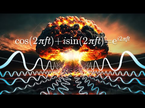
$$e^{i\theta} = \cos\theta + i\sin\theta$$
By multiplying the signal by a complex exponential, the real portion yields the cosine amplitude while the imaginary portion captures the sine amplitude.
- The Earth experiences roughly 300 earthquakes of magnitude 3.0 or greater every 24 hours. - Multiplying out-of-phase or mismatched trial frequencies yields alternating cancellations that average to a net area of zero. - Complex exponentials streamline the calculation of both amplitude and phase shifts in a single mathematical pass.
[10:20](https://www.youtube.com/watch?v=nmgFG7PUHfo&t=620s) The Geneva Seismometer Debate and the Computational Bottleneck
During bilateral technical exchanges at the Geneva summit, the American delegation featured two prominent figures: theoretical physicist Richard Garwin and statistician John Tukey. A technical dispute arose between the delegations regarding whose seismometers possessed greater instrumental precision for monitoring ground motion. Seeking an objective resolution, Garwin took the performance specifications for both sensor designs and ran comparative simulations on a computer at CERN. When he presented the findings the following morning, both delegations conceded that physical hardware differences were essentially negligible.
The realization shifted the focus of the verification effort. The limiting constraint preventing remote identification of underground nuclear explosions was not the physical sensitivity of seismometers, but the processing power required to convert analogue seismic waveforms into digital frequency spectra:
> “The real obstacle to detecting underground explosions wasn't the accuracy of the seismometers, it was the vast amounts of computation required to Fourier transform the seismometer signals.”
Standard Fourier transformation of continuous telemetry required enormous quantities of individual multiplications and additions. For the volumes of continuous seismic data produced worldwide, the calculations overwhelmed the processing capabilities of 1960s computing systems.
[11:00](https://www.youtube.com/watch?v=nmgFG7PUHfo&t=660s) From Continuous Waves to the Discrete Fourier Transform
While theoretical signals can be conceived as infinite, smooth, continuous waves yielding an infinite, continuous frequency spectrum, real-world signals are entirely different. Real data is finite and composed of individual samples or discrete data points. Even when a seismometer trace appears completely continuous and smooth, it does not record ground movement with infinite precision; there is an unavoidable, fundamental graininess to the measurement. Because the available information is discrete and finite, scientists cannot use an idealized Fourier transform and must instead turn to the Discrete Fourier Transform (DFT).
```mermaid flowchart TD accTitle: Continuous versus Discrete Fourier Transform accDescr: Diagram contrasting an idealized continuous signal with a finite sampled signal and its resulting discrete frequency bins.
subgraph Continuous["Continuous Domain"] A["Continuous Wave Signal"] --> B["Continuous Fourier Transform"] B --> C["Infinite Frequency Spectrum"] end
subgraph Discrete["Discrete Domain"] D["Finite Sampled Points (N samples)"] --> E["Discrete Fourier Transform (DFT)"] E --> F["N Discrete Frequency Bins"] end ```
A defining characteristic of the DFT is that the resulting frequency spectrum is likewise discrete and finite, structured into a set of frequency "bins." The spacing and total duration of the samples directly determine the nature of these bins:
- **Sample spacing and maximum frequency:** The wider the gap between samples, the lower the maximum frequency that can be captured, because coarse intervals fail to resolve rapid oscillations. - **Signal duration and resolution:** The shorter the duration of the recording, the harder it becomes to separate nearby frequencies, resulting in wider frequency bins and reduced resolution. - **Fundamental bin:** The lowest measurable non-zero frequency has a period equal to the entire duration of the signal. - **Harmonic bins:** All higher frequency bins are exact integer multiples of that fundamental frequency, fitting two, three, four, or more full periods into the duration of the recording. - **Total bin count:** The total number of frequency bins matches the number of samples ($N$). For example, an eight-sample recording generates eight discrete bins spanning from zero up to seven times the fundamental frequency.
---
[13:00](https://www.youtube.com/watch?v=nmgFG7PUHfo&t=780s) Calculating a DFT and the $O(N^2)$ Bottleneck
To illustrate the mechanics of the standard DFT, consider an eight-sample signal. The transform yields eight distinct bins. The first bin represents a frequency of 0 Hz, which acts as a check for any DC offset—evaluating whether the signal is systematically shifted above or below the x-axis. This is calculated by multiplying each point by 1 and summing them; in this symmetric example, they add up to zero. The second bin evaluates 1 Hz, which fits exactly one full period into the window. Each sample is multiplied by a 1 Hz sine wave and a 1 Hz cosine wave, and the results are summed separately (yielding zero for sine and four for cosine). Repeating this test through 2 Hz, 3 Hz, and so on up to 7 Hz produces the complete spectrum.
While mathematically straightforward, this approach scales terribly on computers. Transforming $N$ data points requires multiplying every point across $N$ different sinusoidal basis waves, demanding $N^2$ complex multiplications.
```mermaid flowchart LR accTitle: Computational Scaling Comparison accDescr: Comparison of computational requirements for standard DFT versus the Fast Fourier Transform across small and large sample sizes.
subgraph Small["8 Samples"] D1["Standard DFT: 64 operations"] F1["FFT: 24 operations"] end
subgraph Large["1,000,000 Samples"] D2["Standard DFT: 1,000,000,000,000 operations (3+ years in 1960s)"] F2["FFT: ~20,000,000 operations (35 minutes in 1960s)"] end ```
For eight data points, 64 calculations is trivial. But for a data set of one million samples, $N^2$ reaches one trillion complex multiplications:
- On 1960s computing hardware, evaluating one trillion calculations for a single transform would require more than three continuous years of run time. - While a single seismic waveform rarely required one million samples, monitoring global compliance required processing tens of events every day from hundreds of independent seismograph stations worldwide. - The brute-force computation created an impossible operational logjam, giving researchers an urgent incentive to discover a shortcut.
---
[14:59](https://www.youtube.com/watch?v=nmgFG7PUHfo&t=899s) A Doodling Mathematician and the Fast Fourier Transform
The critical breakthrough arrived in 1963 during a meeting of the President's Science Advisory Committee (PSAC), attended by President John F. Kennedy along with physicist Richard Garwin and mathematician John Tukey. Despite high-stakes agenda items like the Apollo space program and civil defense nuclear fallout shelters, the proceedings dragged on. Garwin noticed Tukey spent the entire session doodling on his notepad. When the session adjourned, Garwin asked Tukey what he had been sketching and was stunned to discover that Tukey had worked out a radical mathematical shortcut for discrete Fourier transforms. Tukey's method cut down calculations so dramatically that a problem requiring over three years on 1960s computers could run in just 35 minutes.
The resulting method became known as the Fast Fourier Transform (FFT). Instead of performing all $N \times N$ calculations blindly, the algorithm exploits the inherent periodicity and symmetry of sinusoids:
```mermaid flowchart TD accTitle: Fast Fourier Transform Divide and Conquer Strategy accDescr: Flowchart demonstrating how N samples are recursively split into even and odd indices to reduce operations down to N log2 N.
A["All N Samples"] --> B["Split: Even Index Points"] A --> C["Split: Odd Index Points"]
B --> D["Compute lower half frequencies"] C --> E["Compute lower half frequencies"]
D --> F["Exploit Sine/Cosine Symmetries and Twiddle Factors"] E --> F
F --> G["Derive upper half frequencies via reuse"] G --> H["Repeat recursively down to single points: Total O(N log2 N)"] ```
- **Symmetry and overlap:** In the eight-sample scenario, rather than computing 64 distinct products, the waves overlap predictably. At the midpoint sample, all four odd frequencies share identical values, and all four even frequencies also share identical values, collapsing eight multiplications into two. - **First division by two:** Splitting an $N$-point series into even-indexed and odd-indexed samples reveals that, at the sample points, the values of the sine waves for the lower half of frequencies match or are the exact negative of those in the upper half. Thus, solving the lower half yields the upper half almost for free through basic complex multiplication, cutting the workload by half. - **Recursive reduction to $O(N \log_2 N)$:** Applying this split recursively—dividing into even and odd subsets over and over down to isolated individual points—systematically reduces the computational scaling from $O(N^2)$ to $O(N \log_2 N)$. - **Realized computational savings:** For 8 samples, operations drop from 64 down to 24. For 1,000 samples, the algorithm is roughly 100 times faster; for 1,000,000 samples, it requires 50,000 times fewer calculations.
---
[18:52](https://www.youtube.com/watch?v=nmgFG7PUHfo&t=1132s) Cold War Secrecy, Missed Treaties, and Gauss's Lost Discovery
Following Tukey's insight, Richard Garwin approached IBM mathematician James Cooley to program the algorithm on modern computers. Garwin kept the actual national security application strictly hidden; rather than disclosing that the code was intended to pinpoint Soviet underground nuclear detonations, “He said it was to work out the spins in a crystal of helium-3.” Cooley and Tukey subsequently co-authored and published their foundational paper on the algorithm in 1965, sparking an immediate revolution across computer science and digital signal processing.
Tragically, the discovery came slightly too late to salvage negotiations for a Comprehensive Nuclear-Test-Ban Treaty. By 1965, the United Kingdom, France, and China had joined the United States and the Soviet Union in the nuclear club. Because the 1963 Partial Test Ban Treaty banned explosions in the atmosphere, outer space, and underwater but permitted underground testing, governments concluded that failing to test underground would leave them militarily vulnerable:
- **Accelerated testing:** Between 1963 and the mid-1990s, approximately 1,500 nuclear devices were detonated underground—an average cadence of roughly one nuclear detonation every single week for 30 straight years. - **Arsenal expansion:** Global nuclear stockpiles surged to an all-time peak in the mid-1980s of roughly 70,000 active warheads. - **Staggering economic cost:** Inflation-adjusted Cold War nuclear expenditures totaled approximately $10 trillion each for both the United States and the Soviet Union.
When asked whether an earlier deployment of the FFT could have verified low-yield tests and secured a comprehensive ban before the buildup escalated, Dr. Garwin reflected on the near miss:
> “Well, it's a good story.” > > “It would've helped and it might have turned the tide.”
Yet the algorithm had in fact been discovered long before—and simply forgotten. In 1805, Carl Friedrich Gauss was calculating the orbital trajectories of the newly discovered asteroids Ceres, Pallas, and Juno. To determine Juno's path, Gauss invented harmonic analysis methods equivalent to both the Discrete Fourier Transform and Cooley and Tukey's Fast Fourier Transform. His work predated Joseph Fourier's own 1807 paper by two years and Cooley and Tukey's work by 160 years. However, Gauss discarded the method for a different approach and left the work unpublished during his lifetime. The notes only surfaced posthumously in Volume 3 of his collected works, where they lay buried and ignored, transcribed in non-standard mathematical notation and written in 19th-century Latin.
Today, the combination of modern seismological networks, modern computing power, and the FFT enables monitoring agencies to detect seismic events down to magnitude 3.0—equivalent to an explosive yield of merely one kiloton—virtually anywhere across the globe, while the FFT itself serves as the algorithmic engine behind all modern audio, video, and data compression.
[22:10](https://www.youtube.com/watch?v=nmgFG7PUHfo&t=1330s) Image Compression and the Ubiquity of the FFT
The Fast Fourier Transform serves as the foundation for modern image compression techniques. When compressing an image, one takes the pixel brightness values across each row and computes a Fast Fourier Transform. This operation uncovers the specific spatial frequencies present within the brightness variations of those rows. In a visual representation of this transformed data, brightness indicates the magnitude of each frequency component, while color denotes the phase—illustrating how much that frequency is shifted horizontally to the left or to the right. A second FFT is then run down the columns of pixels. The order of operations is completely interchangeable; whether rows or columns are processed first, the end requirement is a two-dimensional FFT of the original image.
```mermaid flowchart TD accTitle: Two-Dimensional FFT Image Compression Pipeline accDescr: Diagram illustrating the steps of taking an original image, computing row and column FFTs, discarding near-zero high-frequency components, and inverting back to view the image.
subgraph Transform["2D Frequency Decomposition"] A["Original Image Pixels"] --> B["Row-wise 1D FFT"] B --> C["Column-wise 1D FFT"] end
subgraph Compression["Data Reduction"] C --> D["2D FFT Matrix"] D --> E["Discard Small High Frequencies<br/>(Up to ~99% of data)"] end
subgraph Reconstruction["Image Retrieval"] E --> F["Compressed File on Disk"] F --> G["Inverse 2D FFT"] G --> H["Reconstructed Image"] end ```
In nearly every real-world photograph, the overwhelming majority of values in the transformed matrix end up extremely close to zero. Although taking the logarithm of these values makes them easier to inspect visually, examining the raw values reveals that the high-frequency components—especially those situated toward the outer edges—are miniscule. This makes it possible to discard up to 99% of the transformed data without significant perceptual loss. When an inverse transform is applied to the remaining data, the rendered picture remains an impressively faithful representation of the original. Consequently, computers routinely store images encoded as two-dimensional transforms and run an inverse FFT whenever the image needs to be viewed.
The impact of the algorithm extends across virtually all modern technology: - **Broad Applications**: Essential for solving differential equations, operating radar and sonar systems, analyzing crystal structures, and transmitting data over Wi-Fi and 5G networks. - **Universal Signal Processing**: The backbone of digital audio, image, and communications workflows. - As the presenter highlights regarding its extraordinary stature, “mathematician Gilbert Strang called the FFT the most important numerical algorithm of our lifetime.” - Had Carl Friedrich Gauss's earlier discovery of the technique been recognized and broadly adopted in his own era, it could have reshaped technological progress even earlier.
[24:11](https://www.youtube.com/watch?v=nmgFG7PUHfo&t=1451s) 80,000 Hours and Maximizing Career Impact
Gauss could not have foreseen how profoundly his mathematical insight would influence the modern world, just as most people rarely reflect on the massive cumulative footprint of their working lives. Over a typical career span—working 40 hours a week, 50 weeks a year, across 40 years—a person spends roughly 80,000 hours on the job. That immense block of time represents the single largest opportunity an individual has to effect positive change in the world.
Standard career guidance from university centers or aptitude batteries tends to be limited; it focuses on personal interests and matching preferences, offering few options beyond traditional callings like teaching or medicine if someone expresses a desire to solve global challenges. Reflecting on this dilemma, the presenter shares his own experience after finishing college: “When I finished college, I knew I liked filmmaking, teaching and science and that I wanted to have a big positive impact but YouTube didn't exist yet and so I honestly had no idea what I was gonna do.” He expresses deep gratitude for landing in a role where he can merge his passions with tangible public benefit, emphasizing that unconventional, impactful paths are out there for others as well.
The video’s sponsor, 80,000 Hours, is a nonprofit organization dedicated to helping individuals identify and pursue careers that address pressing global problems: - **Research Foundation**: Conducted more than a decade of research alongside Oxford University academics to formulate specific, actionable, and evidence-based career advice that moves beyond shallow platitudes like "follow your passion." - **Free Tools & Resources**: Offers an ongoing podcast, research-backed career guides, a newsletter, and an updated job board featuring hundreds of high-impact positions. - **Access**: Everything the nonprofit produces remains permanently free; signing up at `80000hours.org/veritasium` provides immediate digital delivery of their comprehensive career guide.
## Notable quotes > [10:20](https://www.youtube.com/watch?v=nmgFG7PUHfo&t=620s) The real obstacle to detecting underground explosions wasn't the accuracy of the seismometers, it was the vast amounts of computation required to Fourier transform the seismometer signals.
> [06:06](https://www.youtube.com/watch?v=nmgFG7PUHfo&t=366s) If you wanna know how much of a particular sine wave is in a signal, just multiply the signal by the sine wave at each point and then add up the area under the curve.
## Mentioned Fast Fourier Transform, Discrete Fourier Transform, Baruch Plan, Castle Bravo, Daigo Fukuryū Maru, Aikichi Kuboyama, Limited Test Ban Treaty, Comprehensive Nuclear-Test-Ban Treaty, Richard Garwin, John Tukey, James Cooley, Carl Friedrich Gauss, Joseph Fourier, Gilbert Strang, Steve Brunton, Cliff Thurber, Paul Richards, Steven Gibbons, Grant Sanderson, 80,000 Hours, CERN, IBM, President's Science Advisory Committee, John F. Kennedy
## Video description The Fast Fourier Transform is used everywhere but it has a fascinating origin story that could have ended the nuclear arms race. This video is sponsored by 80,000 Hours. Head to http://80000hours.org/veritasium to sign up for their newsletter and get sent a free copy of their in-depth career guide.
A huge thank you to Dr. Richard Garwin for taking the time to speak with us. Thanks to Dr. Steve Brunton of the University of Washington for his help with understanding the Fast Fourier Transform.
Thanks to Dr. Cliff Thurber of the University of Wisconsin-Madison, Dr. Paul Richards of Columbia University, and Dr. Steven Gibbons of the Norwegian Geotechnical Institute for their expertise.
Thanks to Grant Sanderson of 3Blue1Brown for his helpful feedback on the script. His great video on the Fourier Transform is here - https://youtu.be/spUNpyF58BY
▀▀▀ References:
Kristensen, H.M., Korda, M. (2022). Status of World Nuclear Forces. Federation of American Scientists (FAS). https://ve42.co/Stockpile2022
Barth, K. H. (1998). Science and politics in early nuclear test ban negotiations. Physics Today, 51(3), 34-39. - https://ve42.co/Barth1998
Schmalberger, T. (1991). In pursuit of a nuclear test ban treaty - https://ve42.co/Schmalberger1991
Bowers, D., & Selby, N. D. (2009). Forensic seismology and the comprehensive nuclear-test-ban treaty. Annual Review of Earth and Planetary Sciences, 37, 209-236 - https://ve42.co/Bowers2009
Incorporated Research Institutions for Seismology (IRIS). (2022). How Often Do Earthquakes Occur? https://ve42.co/IRIS2022
Kimball, D. (2022). The Nuclear Testing Tally. Arms Control Association. https://ve42.co/TestTally2022
Kværna, T., & Ringdal, F. (2013). Detection capability of the seismic network of the International Monitoring System for the Comprehensive Nuclear Test Ban Treaty. Bulletin of the Seismological Society of America, 103(2A), 759-772 - https://ve42.co/Kvrna2013
Sykes, L. R., & Evernden, J. F. (1982). The verification of a comprehensive nuclear test ban. Scientific American, 247(4), 47-55 - https://ve42.co/Sykes1982
Peterson, J., & Hutt, C. R. (2014). World-wide standardized seismograph network: a data users guide (p. 82). US Department of the Interior, US Geological Survey. - https://ve42.co/Peterson2014
Richards, P. G., & Kim, W. Y. (2009). Monitoring for nuclear explosions. Scientific American, 300(3), 70-77 - https://ve42.co/Richards2009
Jacobsen, L. L., Fedorova, I., & Lajus, J. (2021). The seismograph as a diplomatic object: The Soviet–American exchange of instruments, 1958–1964. Centaurus, 63(2), 277-295 - https://ve42.co/Jacobsen2021
Schwartz S. I. (1998). The Hidden Costs Of Our Nuclear Arsenal: Overview Of Project Findings. The Brookings Institution - https://ve42.co/Schwartz1998
Ricón, J.L. (2016). The Soviet Union: Military Spending. Nintil - https://ve42.co/Nintil2016
Heideman, M. T., Johnson, D. H., & Burrus, C. S. (1985). Gauss and the history of the fast Fourier transform. Archive for history of exact sciences, 265-277 - https://ve42.co/Heideman1985
Ford, D. (2004). Richard Garwin - Session IV. American Institute of Physics (AIP). - https://ve42.co/Ford2004
Aaserud, F. (1986). Richard Garwin - Session I. American Institute of Physics (AIP). - https://ve42.co/Aaserud1986
Goldstein, A. (1997). James W. Cooley, an oral history. IEEE History Center, Piscataway, NJ, USA - https://ve42.co/Goldstein1997
Cooley, J., Garwin, R., Rader, C., Bogert, B., & Stockham, T. (1969). The 1968 Arden House workshop on fast Fourier transform processing. IEEE Transactions on Audio and Electroacoustics, 17(2), 66-76 - https://ve42.co/Cooley1969
▀▀▀ Special thanks to Patreon supporters: Louis Lebbos, Elliot MIller, RayJ Johnson, Brian Busbee, Jerome Barakos M.D., Amadeo Bee, TTST, Balkrishna Heroor, Chris LaClair, John H. Austin, Jr., OnlineBookClub.org, Matthew Gonzalez, Eric Sexton, John Kiehl, Diffbot, Gnare, Dave Kircher, Burt Humburg, Blake Byers, Dumky, Evgeny Skvortsov, Meekay, Bill Linder, Paul Peijzel, Josh Hibschman, Mac Malkawi, Mike Schneider, John Bauer, jim buckmaster, Juan Benet, Sunil Nagaraj, Richard Sundvall, Lee Redden, Stephen Wilcox, Marinus Kuivenhoven, Michael Krugman, Cy 'kkm' K'Nelson, Sam Lutfi, Ron Neal
▀▀▀ Written by Derek Muller & Felicity Nelson Filmed by Derek Muller & Raquel Nuno Animation by Ivy Tello, Jakub Misiek, Alex Drakoulis, and Fabio Albertelli Edited by Albert Leung & Derek Muller Research Assistant: Katie Barnshaw Additional video/photos supplied by Pond5 and Getty Images Music from Epidemic Sound Produced by Derek Muller, Petr Lebedev, and Emily Zhang
[Source](https://www.youtube.com/watch?v=nmgFG7PUHfo)