Sean Parent introduces the central architectural mandate of 'no incidental data structures,' targeting ad-hoc, pointer-based entity relationships that fail to provide a single composite object representing the collection as a whole. (2:23)
Accessing main memory (RAM) is roughly 200 times slower than an L1 cache hit, meaning constant factors and contiguous memory layouts in vector-like structures frequently outperform asymptotically superior algorithms that thrash cache through pointer indirection. (18:39)
Parent critiques the C++ standard's definition of 'valid but unspecified' states after moves or exceptions, arguing that without a preserved semantic invariant, an object is merely in a partially formed state where only assignment and destruction are safe. (7:56)
A physical topological model based on a knotted shoelace and wooden beads demonstrates how to enforce valid tree hierarchies by construction, inspiring the non-intrusive `forest` container in the Adobe Source Libraries (ASL). (43:36)
Detailed notes
## Background
Published on YouTube by CppCon on September 25, 2015, this video features a keynote presentation by Adobe principal scientist Sean Parent. The session examines how standard library containers are frequently misused or underused, showing how ad-hoc, incidental data structures formed by tangled object references can be replaced with well-designed composite containers to drastically simplify software.
## TL;DR
Sean Parent introduces the core architectural goal of eliminating incidental data structures—systems where relationships between objects exist without a single composite entity representing the structure as a whole. Grounding his philosophy in the physical realities of modern memory hierarchies and cache locality, he demonstrates how building blocks like std::rotate and std::nth_element can compose powerful, cache-aware algorithms such as stable partition projections and subrange sorting. He critiques conventional, intrusive UI hierarchies that routinely break regular composite object invariants, introducing instead a non-intrusive 'forest' container inspired by a physical loop of shoelace and beads that makes malformed hierarchies structurally impossible. The lecture concludes by urging engineers to treat the STL as a design pattern for building custom, non-intrusive composite containers that enable local reasoning.
## Atmosphere & style
The presentation combines high-level theoretical rigor with dry, self-deprecating wit and conversational warmth. Parent commands the lecture hall with the effortless authority of a seasoned systems veteran, peppered with teasing banter directed at recognizable peers in the audience like John Lakos and Marshall Clow. A personal narrative about dissecting a toddler's bead toy on the living room floor grounds abstract topology in humorous domestic reality, creating an engaging, intellectually stimulating atmosphere that makes foundational computer science concepts feel immediate and actionable.
## Bulletin
- [02:23](https://www.youtube.com/watch?v=sWgDk-o-6ZE&t=143s) Sean Parent introduces the central architectural mandate of 'no incidental data structures,' targeting ad-hoc, pointer-based entity relationships that fail to provide a single composite object representing the collection as a whole.
- [18:39](https://www.youtube.com/watch?v=sWgDk-o-6ZE&t=1119s) Accessing main memory (RAM) is roughly 200 times slower than an L1 cache hit, meaning constant factors and contiguous memory layouts in vector-like structures frequently outperform asymptotically superior algorithms that thrash cache through pointer indirection.
- [07:56](https://www.youtube.com/watch?v=sWgDk-o-6ZE&t=476s) Parent critiques the C++ standard's definition of 'valid but unspecified' states after moves or exceptions, arguing that without a preserved semantic invariant, an object is merely in a partially formed state where only assignment and destruction are safe.
- [43:36](https://www.youtube.com/watch?v=sWgDk-o-6ZE&t=2616s) A physical topological model based on a knotted shoelace and wooden beads demonstrates how to enforce valid tree hierarchies by construction, inspiring the non-intrusive `forest` container in the Adobe Source Libraries (ASL).
## Key takeaways
- [02:23](https://www.youtube.com/watch?v=sWgDk-o-6ZE&t=143s) A goal in software engineering—like 'no raw loops', 'no raw pointers', or 'no incidental data structures'—is not a dogmatic ban, but an ambitious target that elevates code quality through the discipline of striving toward it.
- [05:13](https://www.youtube.com/watch?v=sWgDk-o-6ZE&t=313s) Semantic relationships bridge arbitrary physical bit patterns to mathematical values and types; losing these semantic invariants leads to invalid values and program safety failures.
- [07:56](https://www.youtube.com/watch?v=sWgDk-o-6ZE&t=476s) The C++ standard's term 'valid but unspecified' is contradictory because an unspecified state lacks semantic meaning; following Alexander Stepanov's formulation, such objects are 'partially formed' and safe only for reassignment or destruction.
- [07:56](https://www.youtube.com/watch?v=sWgDk-o-6ZE&t=476s) Iterator invalidation occurs when the semantic relationship between the iterator and its container's backing storage is severed, even if the iterator's underlying memory bits remain unchanged.
- [13:21](https://www.youtube.com/watch?v=sWgDk-o-6ZE&t=801s) Chapter 12 of 'Elements of Programming' defines regular composite objects via whole-part relationships requiring four invariants: connectivity, non-circularity, logical disjointness, and full ownership.
- [18:39](https://www.youtube.com/watch?v=sWgDk-o-6ZE&t=1119s) Modern hardware memory hierarchies heavily penalize pointer chasing; RAM behaves like a disk drive compared to L1 cache, making contiguous data structures like std::vector the most effective tool in large codebases like Adobe Photoshop.
- [26:41](https://www.youtube.com/watch?v=sWgDk-o-6ZE&t=1601s) The divide-and-conquer implementation of std::stable_partition applies its predicate exactly once per element before any move occurs, which allows position projections across parallel arrays simply by dropping the dereference operator.
- [30:37](https://www.youtube.com/watch?v=sWgDk-o-6ZE&t=1837s) Combining std::nth_element with std::partial_sort yields `sort_subrange`, sorting an arbitrary interior window 2 to 8 times faster than sorting an entire collection by establishing partial spatial order.
- [36:54](https://www.youtube.com/watch?v=sWgDk-o-6ZE&t=2214s) An incidental data structure is any data structure where no single object represents the structure as a whole, common in intrusive UI hierarchies and delegate webs that violate composite object invariants.
- [40:16](https://www.youtube.com/watch?v=sWgDk-o-6ZE&t=2416s) Conventional UI hierarchy implementations using child pointer lists routinely create circular references, non-disjoint sharing, and ownership breakdowns in just a few lines of standard object-oriented code.
- [41:10](https://www.youtube.com/watch?v=sWgDk-o-6ZE&t=2470s) Real-world UI hierarchies are not balanced logarithmic trees but deep, narrow stalks with large leaf clusters (often close to O(n/2) depth), making recursive spatial queries like hit-testing slow compared to dedicated structures like quadtrees.
- [43:36](https://www.youtube.com/watch?v=sWgDk-o-6ZE&t=2616s) A closed loop shoelace threaded through beads provides a physical topology where constructing an invalid or malformed hierarchy without knots is physically impossible, serving as the blueprint for the ASL `forest` container.
- [46:58](https://www.youtube.com/watch?v=sWgDk-o-6ZE&t=2818s) Hierarchical range erasure maps physically to lifting two coordinate points on a shoelace loop: beads whose both loop strands lie within the selection interval fall off naturally, providing a sound model for UI range deletion.
- [56:52](https://www.youtube.com/watch?v=sWgDk-o-6ZE&t=3412s) The ultimate objective of structuring relationships into proper composite containers is to enable local reasoning, allowing engineers to read and understand individual functions in isolation while preserving correctness at system scale.
- [59:14](https://www.youtube.com/watch?v=sWgDk-o-6ZE&t=3554s) There exists a fundamental architectural trade-off between safety and efficiency: high-performance operations require positional semantics like iterators, even if those positions are inherently vulnerable to invalidation.
## Detailed walkthrough
### [00:00](https://www.youtube.com/watch?v=sWgDk-o-6ZE&t=0s) Genesis of the Talk: From C++ Seasoning to a Keynote
Sean Parent introduces himself as a principal scientist at Adobe Systems, where he has worked for just over twenty years across a wide range of projects, focusing recently on mobile digital imaging and web-based imaging systems. Two years earlier, at the GoingNative conference, he delivered a talk titled *C++ Seasoning*, which went on to accumulate more than 100,000 views. In response to widespread audience feedback urging him to write a book based on that presentation, Parent began outlining chapters, using speaking invitations as deadlines to flesh out individual sections. He explains that his original roadmap had a deliberate gap: he had given talks on chapters before and after this topic, but had skipped this one because he considered it merely a "bridge talk" intended to tie the beginning of the book to the end without containing anything flashy.
The path to delivering this material at CppCon began when Jon Kalb invited him to give a keynote on concurrency at Meeting C++ in Moscow, and subsequently asked him to repeat it at C++Now in Aspen. A couple of weeks before C++Now, Kalb emailed Parent asking if he could convert the keynote into a tutorial to fill a conference shortage. Parent agreed, and the session ended up winning awards for both Best Tutorial and Most Useful Talk. Encouraged by that reception, Parent proposed turning this bridge chapter into a tutorial when Kalb asked for a CppCon presentation—only for Kalb to email back announcing that the organizers were so excited about the proposal that they were promoting it to a keynote.
- Sean Parent has spent over two decades at Adobe Systems, contributing to Photoshop and transitioning recently to mobile and web digital imaging.
- *C++ Seasoning* (presented at GoingNative 2013) achieved over 100,000 views online.
- Parent's concurrency tutorial at C++Now in Aspen was voted Best Tutorial and Most Useful Talk.
---
[02:23](https://www.youtube.com/watch?v=sWgDk-o-6ZE&t=143s) Defining the Goal: No Incidental Data Structures
Every chapter in Parent's planned book is organized around a specific target, and the mandate for this keynote chapter is "no incidental data structures." He takes care to contrast a "goal" with strict guidelines or dogmatic rules. Drawing a parallel to his *C++ Seasoning* directives—such as "no raw loops" and "no raw pointers"—he emphasizes that a goal is not meant to be enforced as an absolute prohibition, but rather as an ambitious target that elevates code quality through the sheer discipline of striving to meet it. As Sean Parent puts it, “They're things that by striving to achieve them, your code will get better.”
To clarify what an "incidental" data structure is, Parent first interrogates the textbook definition of a data structure: *a format for organizing and storing data*. While generally acceptable, Parent disputes the requirement for storing data, pointing out that a data structure can exist purely to organize data without necessarily owning or holding the elements internally. Digging deeper into the root concept, a "structure" is simply a collection of things related to other things. Software architects, he observes, are professionals whose entire job is to design these structures by managing relationships between components. However, this reveals a fundamental blind spot in the discipline: “The problem is that computer scientists are very bad at relationships.”
```mermaid
flowchart TD
accTitle: Concept of Data Structure Relationships
accDescr: Diagram illustrating how entities relate via semantic meaning, types, values, and memory addresses.
subgraph Mathematical["Abstract World"]
V["Value (e.g., 4 bananas)"]
T["Type (e.g., int4: -8 to 7)"]
end
subgraph Physical["Physical Machine"]
B["Bits: 0 1 0 0"]
A["Address Space (Spatial & Temporal)"]
end
B -->|"Semantic Relationship"| V
B -->|"Form / Invariant"| T
B -->|"Allocation / Placement"| A
```
---
[05:13](https://www.youtube.com/watch?v=sWgDk-o-6ZE&t=313s) Relationships and Meaning: Semantic, Type, and Value Safety
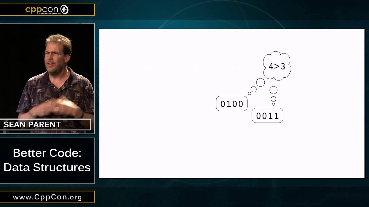
To expose how relationships function in software, Parent conducts a thought experiment starting from absolute nothingness—a dimensionless, void "mythical Haskell space" devoid of width, height, or time. Into this void, he places four bits: `0 1 0 0`. By themselves, these bits carry no intrinsic significance; they gain meaning entirely because the programmer assigns it. They could mean four bananas, the color blue, or the abstract mathematical integer 4. This bridge between raw bits and conceptual significance is a *semantic relationship*. Concurrently, the four bits possess a structural form—a type—which bounds them within a signed range of -8 to 7 simply because the author declared them to be signed rather than unsigned.
These conceptual relationships underpin every modern discussion of software safety. Lifetime safety, type safety, and bound safety are all mechanisms designed to preserve these semantic connections. Parent underscores the severity of breaking these contracts with theatrical gravity: “If we lose the semantic relationship on our type, the universe unravels, missiles launch, it's really bad.” Alongside type safety sits *value safety*, which concerns whether the bit pattern `0 1 0 0` accurately reflects the intended entity of 4. When that connection is broken, value safety fails, and the value is classified as invalid.
---
[07:56](https://www.youtube.com/watch?v=sWgDk-o-6ZE&t=476s) Iterator Validity, "Valid but Unspecified", and Partially Formed States
Parent critiques the C++ standard for employing the term "valid" in two conflicting, problematic ways:
1. **Iterator Validity:** When an iterator references an element inside a `std::vector` and a subsequent `push_back` triggers a reallocation, the standard dictates that the iterator becomes invalid. Crucially, the physical bits representing the iterator in memory have not changed at all; what changed is that the iterator's relationship to the vector's backing storage was severed. Because its meaning has vanished, the object's value is invalid even though its type remains an iterator. The programmer has only two safe options with such an object: restore its semantic meaning by assigning a new value to it, or destroy it.
2. **Move-from States and Exception Guarantees:** In describing the state of an object after a move operation or following an exception under the basic exception guarantee, the standard describes the state as "valid but unspecified." Parent attacks this phrase as a logical impossibility: “Okay, if it's unspecified, it has lost its semantic relationship.” Without an established semantic relationship, an object cannot possess a valid value.
Citing Alexander Stepanov’s formulation in *Elements of Programming*, Parent argues that an object in an unspecified or moved-from state is properly understood as being *partially formed*. Because it lacks an invariant-backed value, the only operations safely permissible on it are re-establishing a meaningful value through assignment or allowing its destructor to run. From this foundation, Parent formalizes fundamental programming concepts:
- **Safe Operation:** “What we mean by a safe operation is an operation that maintains the semantic relationship.”
- **Unsafe Operation:** An operation that risks severing or corrupting that semantic relationship.
- **Type Invariants:** The exact set of properties that must continuously hold true for a value to maintain its validity and semantic meaning.
---
[11:00](https://www.youtube.com/watch?v=sWgDk-o-6ZE&t=660s) Mathematical Structures, Representations, and Address Space
When two entities within a system share the same type and map to the same conceptual space, they can participate in a *value relationship*. For instance, the statement that 4 is less than 3 forms a mathematical, value-based structure. Programmers also construct relationships at the representational level: arbitrary bits in memory can be hashed, compared for equality, or sorted. The hashing of bit representations carries semantic utility exclusively because of the foundational premise that if two objects possess identical representations, they represent identical values. However, Parent reminds the room that the converse is not true: having identical hash values does not guarantee value equality due to collisions.
Ultimately, programmers do not build systems inside an abstract, mythical vacuum; software must execute within a concrete hardware address space. In real memory, an uninitialized integer sitting on the stack is an example of an object in a partially formed state—its bits occupy physical storage, but they possess zero semantic meaning because none was established. In physical hardware, an object’s relationship to its address space is both spatial and temporal: it exists at a particular location *here*, during a specific window of execution *now*. Looking up from his slides, Parent pauses to spot Jon Kalb in the room to demonstrate physical locality in space and time before diving into how these spatial relationships manifest in software structures.
[13:21](https://www.youtube.com/watch?v=sWgDk-o-6ZE&t=801s) Physical, Functional, and Whole-Part Relationships
Sean Parent introduces physical relationships with an in-room joke, pointing out John Lakos and Marshall Clow: “So, John and Marshall are involved in a relationship.” While conventionally described as structural, Parent prefers the term *physical relationship* to avoid muddying the definition of data structures. At the lowest level, two objects in memory have addresses where the address of the first object is strictly less than the address of the second. In isolation, that raw memory order carries zero inherent meaning. However, software can ascribe meaning to it—most notably by sorting the objects. Sorting establishes a direct correlation between the values held by objects and their physical locations in an address space. Parent notes that many modern languages attempt to hide or ignore these physical memory relationships: “We refer to those as the Puritan languages, right? Right. We all know the physical relationships exist, but they're being ignored.”
Moving beyond physical layout, Parent examines *functional relationships*, which arise when a mathematical relationship on values is coupled with a concrete function. For example, adding two numbers to produce seven is a functional relationship, and networks of such relationships form dependency graphs. However, if signed arithmetic overflows, the behavior is undefined and the resulting bits lose any semantic meaning: “It means that my value in my result has no semantic relationship.”
Parent then focuses on the foundational concept of the *whole-part relationship*, referencing Chapter 12 of Alexander Stepanov and Paul McJones's book *Elements of Programming* (EOP). This relationship governs composite objects and requires four strict properties:
- **Connected**: Every part must be reachable starting from the whole composite object (analogous to how a component inside a Honda Civic is physically connected to the car).
- **Non-circular**: An object cannot be a part of itself, directly or indirectly (no circular part chains, even though back-pointers may exist).
- **Logically disjoint**: There can be no mutable sharing. If two wholes share an underlying representation, mutating one must never observe an in-place mutation on the other: “Okay? So there's kind of no mutable sharing that can be allowed.”
- **Ownership**: Copying the whole duplicates all of its parts into completely distinct instances; destroying the whole cleans up every part with it.
Parent emphasizes that these four invariants are precisely what allow composite structures—including standard library containers like `std::vector` and `std::list`—to behave as regular types.
```mermaid
flowchart TD
accTitle: Whole-Part Relationship Properties
accDescr: The four core properties defining regular composite objects according to Elements of Programming Chapter 12.
subgraph WholePart["Whole-Part Invariants (EOP Chapter 12)"]
direction TB
C["Connected: parts reachable from whole"]
NC["Non-Circular: no object is part of itself"]
LD["Logically Disjoint: no mutable sharing"]
OW["Ownership: copy copies parts, destruction frees parts"]
end
WholePart --> Reg["Enables Composite Objects to Be Regular Types"]
```
---
[18:39](https://www.youtube.com/watch?v=sWgDk-o-6ZE&t=1119s) Defining Data Structures and the Modern Memory Hierarchy
Parent provides a formal definition of a data structure: “So a a data structure is a structure utilizing value physical structural and representational relationships to encode semantic relationships on a collection of objects and the choice of encoding can make a dramatic difference in the performance of operations on these objects.” While engineers generally understand algorithmic trade-offs—that indexing a linked list takes linear time while inserting takes constant time, or that a vector trades $O(N)$ insertion for $O(1)$ random access—they frequently underestimate the overwhelming performance impact of the hardware memory hierarchy.
Citing latency data originally compiled by Jeff Dean (and adapted from a presentation by Chandler Carruth), Parent stresses that accessing memory degrades by nearly an order of magnitude at every step away from the core. Accessing main memory takes roughly 200 times longer than accessing an L1 cache line: “On a modern machine, RAM behaves much like a disc drive.” To illustrate why constant factors and cache hits outweigh asymptotic theoretical complexity, he notes that $\log_2(\text{one trillion}) \approx 40$. As a result, an $O(N \log N)$ algorithm running over contiguous, cache-friendly memory often runs significantly faster than a purely linear $O(N)$ algorithm thrashing across disjoint pointer indirections: “Okay can have can be more impacted on its performance by locality of the objects than by the big-O notation on the algorithm. Okay. So locality matters. Use arrays use vectors.”
Parent recalls an online critique from *Lambda the Ultimate* regarding a presentation given either by himself or Chris Cox from the Adobe Photoshop team. The post noted that `std::vector` was by far the number-one data structure used across the entire Photoshop codebase, leading the author to mistakenly conclude that Photoshop lacked sophisticated structural relationships. Parent counters that the opposite is true: the Photoshop team relies heavily on vectors because they deeply understand modern hardware performance.
[22:20](https://www.youtube.com/watch?v=sWgDk-o-6ZE&t=1340s) Implementing Stable Partition with Rotate
To demonstrate how contiguity, parallel arrays, and standard algorithm design intersect, Parent revisits the `gather` algorithm introduced in his earlier *C++ Seasoning* talk (originally developed by Marshall Clow). He recounts a post-talk dinner conversation where an attendee accused him of cherry-picking an unrealistically simple algorithm, arguing: “well algorithms in real life are very complicated... for example you can't write stable partition simply.” Parent's answer: “Yes I can.”
A stable partition reorders a sequence given a unary predicate: all elements that satisfy the predicate ("the good guys") are moved to the front, and those that do not ("the bad guys") move to the back, all while strictly preserving the original relative order within both groups. Rather than using external buffers or complex pointer manipulations, Parent builds a divide-and-conquer implementation from first principles:
1. **Divide**: Split the range into two halves and recursively invoke `stable_partition` on each half.
2. **Merge via Rotate**: This leaves the sequence arranged as `[good_1, bad_1, good_2, bad_2]`. To bring all selected elements together into `[good_1, good_2, bad_1, bad_2]`, the middle section `[bad_1, good_2]` must be swapped while keeping internal orders intact. The audience calls out the exact algorithm required: `std::rotate`. Rotate swaps the adjacent subranges and conveniently returns the boundary iterator between the two sections (the new partition point).
3. **Inductive Basis**: When the recursion bottoms out at a single element, evaluate the predicate on that element. If true, advance the partition point by 1; if false, advance by 0 (leave it at the start).
4. **Boilerplate**: Wrap the logic with checks for empty ranges ($N = 0$) and compute the midpoint offset.
This recursive, divide-and-conquer rotate approach yields a clean, correct, and surprisingly compact implementation of stable partition using standard library concepts.
[26:41](https://www.youtube.com/watch?v=sWgDk-o-6ZE&t=1601s) STL Algorithms as Building Blocks: Stable Partition and Projections
Sean Parent begins by highlighting a unifying design insight behind the Standard Template Library (STL). He observes that almost every component in the STL serves as a foundational building block toward one culminating algorithm: `std::stable_sort`. For example, `std::rotate` is most easily implemented using three calls to `std::reverse`. Interestingly, one can also implement `reverse` in terms of `rotate`, yielding an $O(n \log n)$ version of `reverse` that operates purely on forward iterators—an exercise he leaves to the audience.
Looking closely at the implementation of `std::stable_partition`, Parent points out an extraordinary, counterintuitive property: the predicate is applied exactly once to each element before that element is moved. The algorithm descends all the way to the bottom of its divide-and-conquer tree, reads each object a single time, and then reorganizes the collection on the way back up. This means that by simply stripping out the dereference operator (`*`) where the predicate is invoked, one can create a brand-new algorithm: `stable_partition_position`.
```mermaid
flowchart TD
accTitle: Stable Partition Position Algorithm Flow
accDescr: Parallel arrays where indices project from an integer array to a boolean mask to reorder elements stably.
subgraph Process["Projection Predicate"]
P["Predicate projects iterator in A to index in B<br/>(Reads B[pos] == 1 without touching A's values)"]
end
subgraph Output["Partitioned Result"]
R["Array A: [2, 4, 4, 2, 1, 3, 5, 5, 3, 1]<br/>(Evens preserved in relative order, then odds)"]
end
A --> P
B --> P
P --> R
```
Instead of testing the object’s value directly, the predicate projects an iterator's position in one sequence into a corresponding position in another. Parent illustrates this with two parallel arrays: an array of integers `A` containing `1, 2, 3, 4, 5, 4, 3, 2, 1`, and a boolean mask `B` where true bits correspond to selected (even) values. Running `stable_partition_position` reorders `A` so that all selected elements (`2, 4, 4, 2`) move to the front preserving their relative order, followed by the remaining elements (`1, 3, 5, 5, 3, 1`), without modifying the mask itself.
- This technique decouples UI selection state from core business data, avoiding data pollution and keeping access times fast when selections are irrelevant.
- Selection data can be represented in alternate, memory-efficient formats (such as inversion points indicating ranges) while remaining fully compatible via projection.
- As Sean Parent highlights: “The only place where our predicate is applied is one time to each object before that object's been moved.”
- Changing just that single character creates a powerful tool: “Okay, so just changing that one character, just removing the star in stable partition gave me a new algorithm.”
---
[30:37](https://www.youtube.com/watch?v=sWgDk-o-6ZE&t=1837s) Divide-and-Conquer, Tree Pruning, and `sort_subrange`
Algorithms built around divide-and-conquer strategies generally operate in one of two directions: bottom-up (like `stable_partition`, recursing to the bottom leaves and recombining upward) or top-down (like `quick_sort`, partitioning around a pivot at the top before descending). Both models present massive optimization opportunities through tree pruning: whenever an entire subtree can be proven irrelevant to the final outcome, it can simply be skipped.
```mermaid
flowchart LR
accTitle: Sort Subrange Pipeline
accDescr: Three-step process showing range partitioning via nth_element followed by partial_sort.
Parent poses a concrete problem: given an array of 16 shuffled numbers, how do you sort only an interior window `[SF, SL)` (e.g., indices holding values 6, 7, 8, 9) such that elements appear exactly as if the entire collection had been sorted, without spending time sorting the rest? While audience members suggest `std::partial_sort`, Marshall Clow points out `std::nth_element`. Calling `std::nth_element(F, SF, L)` does two crucial things: it places the correct value at `SF` and partitions the range so that every element preceding `SF` is less than or equal to `*SF`. From there, advancing one element past `SF` and invoking `std::partial_sort(SF + 1, SL, L)` sorts the remaining subrange cleanly.
```cpp
template <typename I> // I models RandomAccessIterator
void sort_subrange(I f, I l, I sf, I sl) {
if (sf == sl) return;
if (sf!= f) {
std::nth_element(f, sf, l);
++sf;
}
std::partial_sort(sf, sl, l);
}
```
- In real-world applications (such as paging through 1,000 document pages, calculating trimmed averages around a median, or scrolling virtualized tables), `sort_subrange` runs roughly 2 to 8 times faster than sorting the entire data set.
- Because `sort_subrange` preserves the partitioning invariants of `nth_element`, extending the sorted window downward to a new boundary `NL` requires only an incremental call to `partial_sort(SL, NL, L)`.
- Parent stresses algorithmic literacy: “So you want to calculate a median quickly with STL. Nth element is how you calculate a median quickly.”
- Explaining the broader principle behind the technique: “What I'm utilizing here is I'm establishing spatial relationships on my object that capture semantic relationships about their value ordering and I'm exploiting that to speed up my algorithm.”
---
[36:54](https://www.youtube.com/watch?v=sWgDk-o-6ZE&t=2214s) Incidental Data Structures and Composite Violations
Moving to the central theme of the lecture, Parent defines an *incidental data structure*: it is a data structure occurring within a system where no single object represents the structure as a whole. In other words, it is a structure formed without a clean whole-part relationship, failing to be a proper composite object.
Incidental data structures introduce severe structural ambiguities, destroy local reasoning, and break value semantics. They proliferate through everyday software patterns like delegates, message handlers, and especially self-referential interfaces. Parent recalls discovering forward declarations in C early in his career, marveling at how a struct could hold a pointer to its own type to construct a linked list. However, this same convenience becomes hazardous when designing APIs.
He examines a typical UI hierarchy API—modeled after the Windows API, stripped of managed C++ quirks:
```cpp
struct Element { /*... */ };
struct ElementCollection {
void add(Element*);
};
struct Panel: Element {
ElementCollection children;
};
```
On the surface, this looks like a straightforward hierarchy. Yet because the interface fails to enforce invariants of ownership and structure, catastrophic topologies easily emerge through simple method calls:
```cpp
Panel p1, p2;
Element e;
p1.children.add(&e);
p1.children.add(&e); // Duplicate insertion: becomes a DAG
p2.children.add(&e); // Multiple parents: DAG with multiple roots
p1.children.add(&p1); // Self-containment: creates an impossible cycle!
```
Parent explains that these are not far-fetched theoretical edge cases; developers inadvertently write these exact patterns in production, leading to bizarre UI states and memory management nightmares. In just four lines of benign-looking code, the system has completely dismantled the definition of a composite object.
- As Sean Parent defines it: “An incidental data structure is a data structure that occurs within a system where there is no object representing the structure as a whole.”
- Emphasizing the hidden danger in everyday APIs, he warns: “We have managed in those four lines of code to violate every property of a composite.”
Continuing his analysis of intrusive UI hierarchy structures, Sean Parent points out how easy it is to break foundational invariants with just a handful of typical object-oriented code statements. Looking at a scenario where a panel contains sub-elements, he demonstrates that the panel can inadvertently end up containing itself, forming a circular reference. Because multiple panels end up sharing the exact same elements, the structures are not disjoint. This directly violates ownership: destructing one panel does not reliably clean up the whole hierarchy. Furthermore, reference-counting mechanisms create retain cycles, completely breaking connectivity.
As Sean emphasizes to the audience, “those four lines of code we violate every principle for a composite object.” While software engineers have universally embraced writing linked lists and dynamically sized arrays as formal container types like `std::vector`, they stubbornly persist in building forests and hierarchies as intrusive, ad-hoc data structures. Programmers embed structural pointers directly inside domain objects, inviting severe structural and algorithmic confusion.
```mermaid
flowchart TD
accTitle: Broken Invariants in Intrusive UI Structures
accDescr: Diagram illustrating circularity, non-disjoint sharing, and broken connectivity in intrusive UI designs.
subgraph ProblematicModel["Intrusive Hierarchy Failures"]
P1["Panel A"] -->|"contains / shares"| E1["UI Element"]
P2["Panel B"] -->|"shares same child"| E1
P1 -->|"contains self"| P1
E1 -.->|"retain cycle"| P1
end
```
[41:10](https://www.youtube.com/watch?v=sWgDk-o-6ZE&t=2470s) The Reality of Hierarchy Shapes and Traversal Pitfalls
The consequences of intrusive hierarchies extend far beyond memory leaks into algorithmic ambiguities. Sean asks what actually happens when iterating over a panel's children: is the iteration merely visiting direct descendants, or is it secretly executing an implicit pre-order depth-first search, or even a post-order depth-first traversal? Because each invoked child node might independently recurse down its own children, the caller has no visibility or control over what algorithmic traversal is taking place.
Sean pushes back forcefully against the common optimization myth that hierarchical tree depth is naturally balanced and logarithmic. In real-world software, especially user interfaces, hierarchies do not fan out gracefully. Instead, they look like deep, narrow stalks terminating in massive horizontal clusters—structures with complexity closer to $O(n/2)$ rather than $O(\log n)$. Using structural containment hierarchies to solve spatial UI questions, such as hit-testing a mouse click by querying deep chains of descendants with “Is it in you? Yes. Okay. Well, check your children bonk bunk bunk all the way down,” is exceptionally slow. Applications should maintain purpose-built parallel data structures like quadtrees for spatial queries rather than forcing containment trees to handle dispatching, and components should communicate directly across the tree instead of endlessly percolating events up and down deep ancestral chains.
- Intrusive representations obscure algorithmic behavior, leaving developers unsure whether child iteration is shallow, pre-order, or post-order depth-first.
- View hierarchies in production are not logarithmic; they tend toward $n/2$ shapes with long vertical containment paths opening into massive clusters of leaf children.
- Spatial queries (e.g., cursor hit-testing) are poorly served by containment trees and should instead utilize dedicated parallel acceleration structures like quadtrees.
- UI event handling routinely degrades when events are forced to percolate up and down containment levels rather than targeting destinations directly.
[43:36](https://www.youtube.com/watch?v=sWgDk-o-6ZE&t=2616s) The Shoelace and Beads: A Physical Model of Hierarchies
To understand how to properly model a hierarchy as a true container, Sean investigates the fundamental nature of positions within data structures. While a sequence of $n$ elements possesses exactly $n + 1$ insertion positions between elements, defining positions within a hierarchy depends heavily on whether it is ordered or unordered, and what "position" formally means. He recounts a foundational breakthrough he had years ago while sitting on the floor with his youngest son, who was playing with a fine-motor-skills toy consisting of wooden beads and shoelaces.
Threaded onto an open string, two beads represent a classic linked list. But Sean noticed that one of the shoelaces was tied into a closed loop at the top. The lace was just thick enough that looping it through a bead filled the bead's hole completely, preventing the string from passing through that bead a second time. However, any segment of loop emerging from a bead could itself be doubled into a sub-loop and passed through another bead, creating an entire nested hierarchy out of a single continuous strand.
Sean was stunned: “I was very excited by this. Like I spent four hours playing with this shoelace and beads.” The loop formed a physical model that could represent sequences and nested structures without knots. Most importantly, the invariant that the model represents a valid hierarchy is built directly into its physical topology. It is physically impossible to construct a malformed, cross-linked, or non-hierarchical graph with this system.
```mermaid
flowchart TD
accTitle: Topological Hierarchy via Shoelace Loop
accDescr: Physical topology of a shoelace loop threading beads into tree nodes without knots.
Knot["Top Knot (Forest Anchor)"]
subgraph Loop["Continuous String Path"]
N1["Bead A (Parent Leading Edge)"]
N2["Bead B (Child Leaf)"]
N1Post["Bead A (Parent Trailing Edge)"]
end
Knot --> N1
N1 --> N2
N2 --> N1Post
N1Post --> Knot
```
[46:58](https://www.youtube.com/watch?v=sWgDk-o-6ZE&t=2818s) Traversal Properties, Structural Invariants, and Range Erase
Exploring the mathematical properties of this shoelace model reveals several operational symmetries:
1. **Forest Handle and Directionality**: The top knot serves as the container handle for the forest, and following the path of the thread imposes a natural, unambiguous directionality.
2. **Stable In-Place Positions**: Every point along the lace represents a valid location to pinch out a new loop and insert a child leaf node without reparenting existing nodes.
3. **Context-Free Iteration**: Any position along the loop uniquely identifies an exact location in the hierarchy without having to allocate or maintain an auxiliary traversal call stack.
4. **Traversal Semantics**: Traversing the lace as it enters the top of a bead represents a pre-order depth-first traversal (leading edge); traversing as it exits out of the bottom yields a post-order depth-first traversal (trailing edge).
The physical model also yields an elegant formulation for range erasure. To erase elements between any two arbitrary iterators in the structure, you simply grab those two coordinate points on the shoelace and pick the whole assembly up in the air: the beads that slide completely off the lace are precisely the nodes that should be deleted. Any bead above your grip toward the top knot cannot fall off; a bead below your fingers only drops away if both strands of the loop pass through your selection interval. Translated directly into code, this produces a clean, mathematically sound implementation for hierarchical UI deletion (such as range selection with Shift-Click in an outline view).
[49:52](https://www.youtube.com/watch?v=sWgDk-o-6ZE&t=2992s) The ASL Forest Container and the Domestic Reality of Computer Science
Sean explains that this shoelace abstraction formed the direct design basis for the `forest` container in the Adobe Source Libraries (ASL). While ASL has aged, Sean actively maintains the container on GitHub where it builds cleanly against modern compilers. Although it is fundamentally a node-based container rather than a cache-dense array, it provides an invaluable guarantee: “it has this wonderful safety attribute that I can't create a non-hierarchy.” Iterators explicitly distinguish leading from trailing edges, eliminating all ambiguity over pre-order versus post-order range scans.
Bringing the story full circle, Sean shares an anecdote from two weeks prior to the talk. His wife was babysitting, using an old toy chest kept from when their children were young—his youngest son now being 26 years old. Inside was the very bag containing the original beads and shoelaces. Sean was thrilled: “I had this very humorous thought that it's like, well, someday maybe in computer history museum next to Martin Newell's teapot there will be Sean's shoelace.” He asked his wife if he could take the laces and beads to the conference to show his audience, explaining how they represented an elegant model of hierarchical data structures. His wife, a nurse, stared back at him with an expression closer to disgust than awe, snatched the beads away, and remarked, “That's what you remember?” Sean jokes dryly to the laughing room, “So computer scientists, we're bad at relationships.”
He wraps up this section with concrete directives for software design:
- Programmers must master and respect the structural realities dictated by entity relationships.
- Structural invariants must be encapsulated strictly within composite container types rather than distributed across intrusive member pointers.
- Developers should leverage existing tools in the standard library and actively create robust, non-intrusive container alternatives whenever complex structures are required.
[53:16](https://www.youtube.com/watch?v=sWgDk-o-6ZE&t=3196s) The Role of the STL and Concluding Remarks
Sean Parent closes the lecture portion of his talk by urging engineers not to treat the standard library as an untouchable black box, but rather to look deep inside it. Developers should read the interfaces, study how they are implemented, and understand how they would write those components themselves. He emphasizes that the Standard Template Library (STL) is fundamentally an instructional guide: “STL is intended to be an example.” It is not meant to be a beginning or an end, but an illustration of how to structure code properly. He reiterates the guiding philosophy of the session: eliminate incidental data structures, embrace composite types, and write better code.
[54:09](https://www.youtube.com/watch?v=sWgDk-o-6ZE&t=3249s) Q&A: Learning from Library Implementations and the Rotate Algorithm
An audience member asks where to look for modern C++ libraries that best demonstrate the clean architectural properties Parent discussed, noting that standard library sources shipping on modern machines can be difficult to learn from. Parent agrees completely, explaining that system STL implementations are heavily "munched" and hyper-optimized, making them nearly impossible to plow through for educational purposes. Instead, he often revisits Alexander Stepanov's classic SGI STL source code online to see clear, understandable algorithm designs. He also recommends Stepanov's online course notes as a more approachable entryway than the denser masterpiece *Elements of Programming* (EoP).
Parent highlights that many classic algorithms still offer opportunities for re-evaluation against modern hardware architectures:
- `std::rotate` has three distinct implementations conditioned on iterator concepts: forward, bidirectional, and random access.
- On modern hardware, hardware prefetching heavily favors linear forward memory access: Parent hypothesizes that the forward iterator implementation of `rotate` might actually outperform the bidirectional iterator version—which walks backwards across memory like a physical disk drive seeking in reverse—and could potentially even beat the random access variant.
- When asked if he plans to publish a book similar to Stepanov's *Notes on Programming*, Parent jokes that the only task left is writing it; he has accumulated vast material through teaching, lecture notes, and conference talks, but acknowledging the immense effort required, he confirms: “So yes I would like to get a book out.”
[56:52](https://www.youtube.com/watch?v=sWgDk-o-6ZE&t=3412s) Q&A: Code as Data Structures and Reasoning Locally
An attendee presents a hypothesis: can code itself (call graphs, instruction streams, raw loops with loop variables and iterators) be viewed as an incidental data structure, meaning the rules for good code directly mirror the rules for good data structures? Parent wholeheartedly agrees, pointing out that the term *incidental data structure* was originally coined by Professor Jaakko Järvi at Texas A&M in a collaborative research paper on property models, which modeled dependency graphs and dataflow in applications.
Parent explains that large software systems are webs of different relationship types:
- Functional relationships
- Value relationships
- Structural relationships
- Representational relationships
- High-level whole-part relationships
```mermaid
flowchart TD
accTitle: System Relationships and Local Reasoning
accDescr: Diagram illustrating how architectural relationships lead to modular local reasoning.
subgraph Relationships ["Code & Data Relationships"]
R1["Functional & Value"]
R2["Structural & Representational"]
R3["Whole-Part Hierarchies"]
end
subgraph Reasoning ["Architectural Goal"]
G1["Modular Function Design"]
G2["Reason Locally About Code"]
G3["Predictable Behavior at Scale"]
end
Relationships --> G1
G1 --> G2
G2 --> G3
```
Parent explains that managing these relationships cleanly is the core point of every chapter in his Better Code series: “So if you look at every single chapter in here, what the punchline is is how do I get my code in the point where I can sit down with one function and read that function and understand what in the world is going on with my code.” When relationships are structured so that code can be understood locally, the system will reliably work at scale.
[59:14](https://www.youtube.com/watch?v=sWgDk-o-6ZE&t=3554s) Q&A: Hierarchical Data Locality and Iterator Safety Trade-offs
A listener asks how to reconcile Parent’s call for hardware-friendly cache locality with the tree-like `forest` container he presented, which was implemented as a node-based data structure. Parent acknowledges the tension:
- He has not yet implemented a contiguous-memory cache-friendly forest, though he believes it is entirely doable and worth exploring.
- Traditional node-based structures can mitigate cache thrashing by using custom arena or pool allocators to keep node allocations contiguous.
- When the audience member points out a hardcoded `delete` statement in the presented forest slide, Parent concedes that the current version might not fully support an allocator parameter, though retrofitting allocator support into it would be straightforward.
Another audience member asks whether the fragile relationship between iterators and containers represents an incidental data structure that ought to be eliminated. Parent clarifies that iterator fragility is inherent to positions:
- “Recently I wrote a little blog post about move that you can find online that I think has a beautiful little proof that says that there's a fundamental tradeoff between safety and efficiency.”
- Iterator invalidation makes them inherently unsafe, but "unsafe" is not synonymous with bad; absolute safety and peak performance are fundamentally at odds.
- High-level abstractions like Eric Niebler's Ranges library significantly improve the ergonomics and safety of iterating over ranges without abandoning performance.
- Ultimately, positions within data collections inevitably exist; operations like `rotate` intrinsically require an internal division point (midpoint) within a bounded range.
Parent wraps up the session by noting that this was the premiere run of this specific talk, thanking the audience, and soliciting feedback, corrections, and slide typo reports before the conference breaks.
## Notable quotes
> [36:54](https://www.youtube.com/watch?v=sWgDk-o-6ZE&t=2214s) An incidental data structure is a data structure that occurs within a system where there is no object representing the structure as a whole. — Sean Parent
> [18:39](https://www.youtube.com/watch?v=sWgDk-o-6ZE&t=1119s) On a modern machine, RAM behaves much like a disc drive. — Sean Parent
> [02:23](https://www.youtube.com/watch?v=sWgDk-o-6ZE&t=143s) The problem is that computer scientists are very bad at relationships. — Sean Parent
> [07:56](https://www.youtube.com/watch?v=sWgDk-o-6ZE&t=476s) What we mean by a safe operation is an operation that maintains the semantic relationship. — Sean Parent
## Mentioned
Sean Parent, Adobe Systems, Photoshop, Jon Kalb, Marshall Clow, John Lakos, Chris Cox, Jeff Dean, Chandler Carruth, Alexander Stepanov, Paul McJones, Jaakko Järvi, Eric Niebler, Martin Newell, Elements of Programming, Notes on Programming, Adobe Source Libraries, SGI STL, Ranges, Google, Chrome OS, Apple, PowerPC, CppCon, C++Now, Meeting C++, GoingNative, Lambda the Ultimate, Texas A&M University
## Video description
http://www.cppcon.org
--
The standard library containers are often both misused and underused. Instead of creating new containers, applications are often structured with incidental data structures composed of objects referencing other object. This talk looks at some of the ways the standard containers can be better utilized and how creating (or using non-standard library) containers can greatly simplify code. The goal is no incidental data structures.
--
Sean Parent is a principal scientist and software architect for Adobe’s mobile digital imaging group. Sean has been at Adobe since 1993 when he joined as a senior engineer working on Photoshop and later managed Adobe’s Software Technology Lab. In 2009 Sean spent a year at Google working on Chrome OS before returning to Adobe. From 1988 through 1993 Sean worked at Apple, where he was part of the system software team that developed the technologies allowing Apple’s successful transition to PowerPC.
--
Videos Filmed & Edited by Bash Films: http://www.BashFilms.com
Work at Hudson River Trading (HRT): https://tinyurl.com/safxfctf
## Background
本视频由 CppCon 官方频道于 2015 年 9 月 25 日发布在 YouTube 平台上,记录了 Adobe 首席科学家 Sean Parent 在 CppCon 2015 大会上的主题演讲。演讲简介指出,标准库容器常常既被误用又被低估,应用开发中普遍充斥着由对象间指针引用所拼凑出的“偶发数据结构”,本次分享旨在探讨如何更好地利用标准容器并构建正规容器来简化代码,核心目标是彻底消除偶发数据结构。
## TL;DR
Sean Parent 深入剖析了语义关系、物理内存布局与现代硬件缓存层级对软件性能的决定性影响,呼吁开发者停止编写破坏“整体-部分”(Whole-Part)关系的侵入式自引用结构。演讲以算法推导开篇,现场展示了如何利用连续内存配合 `std::rotate` 构建优雅高效的 `stable_partition` 及 `sort_subrange` 算法。随后,Sean 讲述了他从陪伴儿子玩耍的“鞋带与木珠”物理模型中获得灵感的过程,阐释了树形层次结构的不变式如何自发成立,并展示了其在 Adobe Source Libraries(ASL)中开源的 `forest` 容器。最后他强调,优秀的架构必须将结构不变式封装进复合类型中,从而实现对局部代码的独立推理能力。
## Atmosphere & style
整场演讲兼具深厚的数学哲学思辨与风趣幽默的工程洞察。Sean Parent 登台从容笃定,娓娓道来,从虚拟无维度的纯粹比特空间跨越到物理硬件与现代缓存的残酷现实,理论推演环环相扣。现场互动极为热烈,不论是调侃台下同行间的“物理关系”,还是用妻子对自己沉迷“鞋带算法”的白眼自嘲程序员不擅长处理人际关系,都引来全场阵阵欢笑,让原本枯燥硬核的数据结构设计变得生动而富有温情。
## Bulletin
- [02:23](https://www.youtube.com/watch?v=sWgDk-o-6ZE&t=143s) Sean Parent 提出了本次演讲的核心目标:“消除偶发数据结构”(No incidental data structures),强调应通过显式复合对象封装系统组件间的不变量与所有权关系,而非通过指针与引用任意交织构建隐式图结构。
- [18:37](https://www.youtube.com/watch?v=sWgDk-o-6ZE&t=1117s) 现代硬件的内存层级对性能产生颠覆性影响:主内存(RAM)的访问延迟已高达 L1 缓存的 200 倍以上,其行为特征近乎机械硬盘,数据局部性(Data Locality)对性能的实际制约往往远超过纯理论算法的时间复杂度差异。
- [26:41](https://www.youtube.com/watch?v=sWgDk-o-6ZE&t=1601s) 通过对标准分治算法中解引用操作的剥离,Sean Parent 推导出基于位置投影的衍生算法 stable_partition_position,实现了将 UI 选择状态与核心业务数据解耦的高效重排。
- [43:36](https://www.youtube.com/watch?v=sWgDk-o-6ZE&t=2616s) 基于单根闭合环状鞋带穿过木珠的物理玩具模型,Sean 设计了 Adobe Source Libraries (ASL) 中的 forest 树形容器,从物理模型和拓扑结构上杜绝了非层次结构、环路及多父节点等脏状态的产生。
## Key takeaways
- [02:23](https://www.youtube.com/watch?v=sWgDk-o-6ZE&t=143s) “目标”(Goal)不同于死板的规则(Rule),它是持续追求的工程导向,如同“不用裸循环”和“不用裸指针”一样,通过追求达成能够系统性提升代码质量。
- [05:13](https://www.youtube.com/watch?v=sWgDk-o-6ZE&t=313s) 数据与对象在计算机中通过语义关系赋予现实意义,而类型安全、生命周期安全与边界安全的根本目的均在于持续守护这种语义关系不发生断裂。
- [05:13](https://www.youtube.com/watch?v=sWgDk-o-6ZE&t=313s) C++ 标准中对“valid but unspecified”(有效但未指定)的定义存在语义矛盾,在 Alexander Stepanov 的理论中该状态被更准确地定义为“部分形成状态”(partially formed state)。
- [13:21](https://www.youtube.com/watch?v=sWgDk-o-6ZE&t=801s) 现代许多高级语言试图隐藏对象的物理内存地址关系(被戏称为“清教徒语言”),但诸如排序等操作的本质正是将对象的语义大小映射到底层内存地址的先后拓扑中。
- [16:32](https://www.youtube.com/watch?v=sWgDk-o-6ZE&t=992s) 根据《Elements of Programming》,构成正则复合对象的“整体-部分关系”必须严格遵循四大支柱:连通性(Connected)、非循环性(Non-circular)、逻辑上不相交(Logically disjoint)以及独占所有权(Ownership)。
- [18:37](https://www.youtube.com/watch?v=sWgDk-o-6ZE&t=1117s) 由于现代多核架构中 RAM 访问延迟相较 L1 缓存暴增 200 倍以上,Photoshop 等大型商业软件在架构设计中第一优先级采用 std::vector 以充分榨取硬件缓存局部性。
- [22:20](https://www.youtube.com/watch?v=sWgDk-o-6ZE&t=1340s) std::stable_partition 的分治推导可以通过两次递归划分配合一次原地 std::rotate 算法极简实现,并自然输出划分点。
- [26:41](https://www.youtube.com/watch?v=sWgDk-o-6ZE&t=1601s) 从 stable_partition 中移除谓词的解引用操作可以衍生出 stable_partition_position,利用布尔掩码以极低开销对外部数据完成基于位置的稳定聚集操作。
- [30:37](https://www.youtube.com/watch?v=sWgDk-o-6ZE&t=1837s) 利用 std::nth_element 的快速选择与附带空间划分性质,结合 std::partial_sort 可以剪除分治树分支,构建出比全排序快 2 到 8 倍的 sort_subrange 局部排序算法。
- [36:54](https://www.youtube.com/watch?v=sWgDk-o-6ZE&t=2214s) “偶发数据结构”指的是在缺乏显式整体对象(整体-部分关系)的情况下,由各对象自引用交织形成的隐式结构,容易使树形层级悄然退化为多根 DAG 甚至死锁环状图。
- [40:16](https://www.youtube.com/watch?v=sWgDk-o-6ZE&t=2416s) 真实的 UI 视图层级通常呈现扁平发散形态(深度接近 N/2),采用侵入式父子指针做事件冒泡与命中测试效率低下,应使用四叉树等平行的辅助索引结构进行解耦通信。
- [43:36](https://www.youtube.com/watch?v=sWgDk-o-6ZE&t=2616s) 单根打结鞋带穿过木珠的模型天然内置了层次结构不变式,其下行与上行遍历直接对应先序与后序深度优先遍历,两指悬空提起的区间删除模型直接映射了树控件的批量删除几何逻辑。
- [49:52](https://www.youtube.com/watch?v=sWgDk-o-6ZE&t=2992s) Adobe Source Libraries (ASL) 中的 forest 容器将树形层次关系从侵入式指针抽离为标准化独立容器,在类型系统层面彻底消除了非法非层次状态的出现可能。
- [53:16](https://www.youtube.com/watch?v=sWgDk-o-6ZE&t=3196s) STL 的核心定位不是现成工具的终点,而是指导编写优秀规范代码的范例;阅读 Stepanov 的 SGI STL 早期纯粹实现有助于深入理解算法结构与泛型范式。
- [56:52](https://www.youtube.com/watch?v=sWgDk-o-6ZE&t=3412s) 消灭隐式依赖与偶发数据结构的核心目的,是让工程师能够对单一函数实现“局部推理”(reason locally),保证系统在规模扩张时的健壮可维护性。
- [01:00:52](https://www.youtube.com/watch?v=sWgDk-o-6ZE&t=3652s) 在系统架构中,安全(Safety)与极致效率(Efficiency)之间存在着不可兼得的天然数学权衡,Ranges 抽象虽然提升了迭代器成对操作的安全性,但断点操作仍需触碰内部位置。
## Detailed walkthrough
### [00:00](https://www.youtube.com/watch?v=sWgDk-o-6ZE&t=0s) 演讲缘起与成书计划
Sean Parent 开场介绍了自己的背景:他是 Adobe 公司的 Principal Scientist(首席科学家),在 Adobe 已经任职超过 20 年。他近年来主要专注于移动数字图像处理(Mobile Digital Imaging)以及一些基于 Web 的数字图像处理,他认为这些工作非常吸引人。两年前,他在 GoingNative 大会上做了一场名为《C++ Seasoning》的演讲。现场询问观众时,许多人都举手表示看过。Sean 提到那个演讲在网上的播放量已经突破 10 万次,反响极为热烈,许多人甚至建议他基于该演讲写一本书。
```mermaid
flowchart LR
accTitle: Sean Parent Book Chapters and Talks
accDescr: 演讲内容如何对应到 Sean Parent 正在构思的技术书籍章节。
subgraph S1["书籍构思体系"]
A["《C++ Seasoning》等早期演讲"] --> B["《Better Code: Data Structures》 (过渡章节)"]
B --> C["并发等后期演讲 (已讲内容)"]
end
B --> D["最终目标:成书《Better Code》"]
```
于是,Sean 开始为这本书拟定章节大纲。他的策略是:每次受邀做技术演讲,就把书中的某一个章节充实并讲出来,希望假以时日能把整本书写完。对于今天讲的这一章,关注过他以往分享的人可能会感到好奇,因为他之前已经讲过这个节点之后的章节(如并发),也讲过之前的章节,唯独跳过了这一章。Sean 坦言,这章其实是一个“过渡章节”(bridge talk),负责把书的前半部分和后半部分串联起来,他原本觉得这章平淡无奇,没有什么特别引人注目的东西值得单独做演讲。
- 演讲者:Sean Parent,Adobe 首席科学家,在 Adobe 工作逾 20 年。
- 背景演讲:《C++ Seasoning》(GoingNative 2013),全网观看量超 10 万次。
- 演讲的性质:正处于撰写中的新书里的一个承上启下的过渡章节。
---
### [01:25](https://www.youtube.com/watch?v=sWgDk-o-6ZE&t=85s) 从教程到主题演讲的意外演变
该话题之所以最终登上 CppCon 的讲台,源于一段充满戏剧性的邀请过程。去年 2 月,Sean 受邀在莫斯科举行的 Meeting C++ 大会上做了关于并发(Concurrency)的 Keynote 演讲。会议结束后,Jon Kalb 联系他,询问能否在阿斯彭(Aspen)举办的 C++Now 大会上重复那场并发演讲,Sean 欣然答应。然而就在会议开幕前两周,Jon 突然发来邮件求助:“Sean, we're short on tutorials. Can you give that keynote as a tutorial?”(Sean,我们这边的教程环节缺人,你能把那个主题演讲改成教程形式来讲吗?)。
Sean 答应了请求并进行了调整,结果反响极好,还一举斩获了当届大会的“最佳教程奖”(Best Tutorial)和“最实用演讲奖”(Most Useful Talk)。随后,Jon 再次抛出橄榄枝,询问他是否愿意在 CppCon 上发表演讲。Sean 想到,既然教程形式反响不错,那么书中这个充当桥梁的章节非常适合以教程的形式呈现,于是便提交了选题。没过多久,他又收到了 Jon 的邮件:“We're very excited about your talk. We're going to make it a keynote.”(我们对你的演讲感到非常兴奋,我们决定把它升格为主题演讲)。Sean 在台上打趣道:“So thanks, John.”(所以,多谢了,Jon)。
- 2015 年 2 月:在莫斯科 Meeting C++ 发表并发主题演讲。
- C++Now(Aspen):临时由 Keynote 改为 Tutorial,获得“最佳教程奖”与“最具实用价值演讲奖”。
- CppCon 2015:原本计划作为普通技术教程(Tutorial)提交,最终被大会组织者 Jon Kalb 提升为 Keynote 主题演讲。
---
### [02:23](https://www.youtube.com/watch?v=sWgDk-o-6ZE&t=143s) 核心目标:消除偶发数据结构
Sean 指出,他这本正在写作的书里,每一个章节都会树立一个明确的“目标”(Goal)。本章的核心目标就是:“No incidental data structures”(消除偶发数据结构)。他特别强调,“目标”(Goal)这个词是经过深思熟虑专门挑选的,它与准则(Guideline)或硬性规则(Rule)有着本质区别。目标往往极其难以百分之百达成。正如他在《C++ Seasoning》中提出的“No raw loops”(不用裸循环)和“No raw pointers”(不用裸指针)一样,这些都不是死板的禁令,而是需要工程师不断追求的境界。Sean 阐述了这一设定的核心逻辑:“They're things that by striving to achieve them, your code will get better.”(通过努力去实现它们,你的代码就会变得更好)。
为了搞清楚什么是“偶发数据结构”,首先必须退一步思考:到底什么是数据结构?大家平时的第一反应通常是诸如 `std::list`、`std::vector`、`std::map` 这些具体的容器类。字典或权威资料通常将数据结构定义为“组织和存储数据的格式”(a format for organizing and storing data)。Sean 对后半句提出了异议:他认为数据结构完全可以仅仅是一种用于“组织”数据的格式,数据本身并不一定要存储在数据结构的内部。然而这个定义依然让人觉得不够透彻,因为它并没有解释清楚究竟什么是所谓的“格式化”和“组织”。
进一步拆解这个词,就需要探究什么是“结构”(Structure)。在本质上,“结构”就是事物与其他事物之间的关联与联系(things that are related to other things)。Sean 环视台下,询问有多少人的职位头衔带有“架构师”(Architect)字样。他解释道,架构师的本职工作就是设计结构(designs structures)。换句话说,架构师真正关心的,是软件系统中各个组件彼此之间的关系。但这里存在一个根本性的冲突,正如 Sean 犀利幽默的论断:“The problem is that computer scientists are very bad at relationships.”(问题在于,计算机科学家非常不擅长处理关系)。
- 章节目标:消除偶发数据结构(No incidental data structures)。
- “目标”与“规则”的差异:目标是持续努力的方向,驱动代码演进,而非生硬死板的条规。
- 类似经典目标:在《C++ Seasoning》中提出的“不用裸循环”、“不用裸指针”。
- 软件架构师的核心职责:关注并设计系统组件之间的相互关系。
---
### [05:13](https://www.youtube.com/watch?v=sWgDk-o-6ZE&t=313s) 语义关系、类型系统与安全性的本质
为了从哲学和数学高度审视这种关系,Sean 在屏幕上展示了一张纯空白的幻灯片。他用略带神秘的口吻描述:这张幻灯片代表了字面意义上的“虚无”(nothing / void)——这里没有宽度、没有高度、没有时间维度,是一个毫无维度的虚构 Haskell 空间(mythical Haskell space)。在这个空间里漂浮着 4 个比特位(bits):`0 1 0 0`。它们无始无终,一直存在于那里。
```mermaid
flowchart TD
accTitle: Relationships of Bits in Pure Space
accDescr: 比特、语义含义、类型范围以及表示之间的关系映射。
subgraph Concept["抽象概念与空间"]
Bits["比特位: 0 1 0 0"]
Semantic["语义实体: 4 (香蕉 / 蓝色 / 纯数)"]
TypeRange["类型与范围: [-8, 7] (有符号)"]
HashVal["表示形式: Hash / 逐位表示"]
end
Bits -->|"赋予语义关系"| Semantic
Bits -->|"赋予形式与类型约束"| TypeRange
Bits -->|"底层内存映射"| HashVal
```
Sean 指出,这 4 个比特代表“4 根香蕉”,或者代表“蓝色”,抑或代表抽象数字“4”。它们之所以能代表这些,纯粹是因为“我赋予了它们这个含义,我认为它们就是这个意思”——这就是**语义关系**(semantic relationship)。这些比特位与现实或抽象的实体建立了关联。不仅如此,这 4 个比特作为一个整体还具有形式,即**类型**(Type)。例如,它们映射到有符号范围 $[-8, 7]$。观众可能习惯性认为它们是无符号的,但 Sean 强调这依然是由设计者定义的规则:“Because I said so. Okay, this is my universe.”(因为我说了算。好,这就是我的宇宙)。
这些关系至关重要。在此前的演讲中,Herb Sutter 谈到了类型安全(Type safety)、生命周期安全(Lifetime safety)和边界安全(Bounds safety),其实归根结底都是在守护这种语义关系。如果类型上的语义关系断裂,“宇宙就会分崩离析,导弹就会升空,后果极其严重”。同样,系统还存在**值安全**(Value safety),即比特位是否真实有效地代表了它所宣称的值。一旦失去这一层关系,值就变成了**无效值**(invalid value)。
此时 Sean 展开了对概念严谨性的剖析:在 C++ 语言标准中,“valid”(有效)这个词实际上在两个相互矛盾的语境下被使用:
1. **迭代器失效(Iterator validity)**:如果一个迭代器指向 `std::vector` 中的元素,随后调用 `push_back` 导致底层的动态数组重新分配内存并迁移,该迭代器即宣告失效(invalid)。迭代器本身的比特位并没有发生改变,但它与原 vector 容器之间的关系被切断了,意义随之丢失。这种失效对象唯一的合法出路,要么是通过赋值重新建立关联赋予其意义,要么直接走向析构。
2. **移动后状态与基本异常保证(Moved-from state & Basic exception guarantee)**:标准在描述对象被 move 之后,或者在抛出异常满足基本异常保证时,使用了“valid but unspecified”(有效但未指定)这一表述。Sean 直截了当地指出这是自相矛盾的:“That's a contradiction. If it's unspecified, it has lost its semantic relationship. It is no longer a valid value.”(这是自相矛盾的。如果是‘未指定’的,它就已经失去了语义关系。它不再是一个有效的值)。在 Alexander Stepanov 的经典著作《Elements of Programming》(编程原本)中,这种状态被准确地定义为**部分形成状态**(partially formed state)。
因此,软件领域关于安全与不安全的界定变得清晰起来:所谓**安全操作**,就是能够完整维持语义关系的操作;而**不安全操作**,就是可能斩断语义关系的操作。所谓**类型不变量**(Invariants on a type),本质上就是为了保证该值持续有效、维系其固有含义而必须始终成立的数学与逻辑性质。
- 语义关系(Semantic relationship):抽象数据(比特)与实际现实概念(如香蕉、颜色、数字)之间的映射。
- 值的安全性:保护比特表达的意义不发生偏离;失去语义即为无效(invalid)。
- C++ 标准中关于 Valid 概念的冲突:
- 迭代器失效:比特没变,但因与宿主容器关系断裂而失效。
- 移动后状态(Moved-from):标准称为“valid but unspecified”,Sean 认为这在语义上已失去确定意义,实际上处于无效状态(部分形成状态)。
- Alexander Stepanov 的术语定义:被移走或未确定值的对象实质处于“部分形成”(partially formed)状态。
---
### [11:00](https://www.youtube.com/watch?v=sWgDk-o-6ZE&t=660s) 值关系、表示关系与物理内存地址空间
讨论继续深入。如果空间中存在两个同类型且映射到相同空间的对象,就能在它们之间建立起**值关系**(Value relationship)。比如,判定 $4 < 3$(或者 $3 < 4$),这是一种基于值的数学结构(mathematical structure / value-based structure)。
除了基于值的抽象逻辑,还可以纯粹根据比特表示来建立**表示关系**(Representational relationship)。例如,可以直接对内存中的比特进行哈希(Hash)运算,或者比较比特是否完全相等。哈希之所以有意义,依据的是一个基础前提假设:如果两个对象具有相同的比特表示,那么它们就代表相同的值。这就是将底层的表示关系映射到了高层的值关系,赋予了哈希实际的工程意义。然而其逆命题并不必然成立:哈希相等并不意味着两者的值一定相等(存在哈希碰撞)。
然而,程序员终究无法永远活在那个脱离现实的纯数学神话空间里,代码必须落地于物理现实:
```mermaid
flowchart LR
accTitle: Object in Address Space
accDescr: 对象在物理地址空间中所具有的时空关系。
subgraph Memory["内存地址空间 (Address Space)"]
Obj["对象实体: 0 1 0 0"]
Raw["未初始化内存 / 无语义比特"]
end
Obj -->|"空间关系"| Addr["物理内存地址"]
Obj -->|"时间关系"| Time["对象生命周期 (此时此刻)"]
```
现实世界是**地址空间**(Address space)。在栈上随意分配一个未初始化的整型变量(uninitialized integer),那段内存里的比特位没有任何语义含义,因为它从未被赋予意义。它处于典型的“部分形成状态”,唯一能对它做的安全操作,就是赋予一个新值来建立意义,或者任由其随着作用域结束而销毁。一旦一个对象被放置在真实的地址空间内,它就与该空间建立起紧密联系——那就是**对象的内存地址**。这是一种交织了空间与时间的双重关系:这个具体对象“此时此刻正位于此处”(This object is here now)。讲到这里,Sean 视线扫向观众席寻找主办方 Jon,以确认他的位置作为现实空间关系的生动类比。
- 值关系(Value relationship):建立在值域之上的抽象数学关系,如数值大小比较。
- 表示关系(Representational relationship):底层比特级别的哈希或逐位对比。
- 地址空间与物理现实:
- 纯抽象空间脱离了硬件限制,现实中对象存在于具体的内存地址空间中。
- 未初始化的栈变量属于无语义的“部分形成状态”。
- 内存地址不仅代表空间位置(Spatial),还代表对象的生命周期与时间状态(Temporal)。
### [13:21](https://www.youtube.com/watch?v=sWgDk-o-6ZE&t=801s) 物理关系、函数关系与“清教徒语言”的盲区
Sean Parent 指向台下的听众开玩笑,提到了 John 和坐在后排的 Marshall Clow。他调侃称 John 和 Marshall 之间存在某种“关系”。通常人们会称之为“结构关系”(structural relationship),但因为本场演讲的核心目标就是要为“结构”下定义,所以他将其改称为“物理关系”(physical relationship)。接着 Sean 笑着向全场打趣,称大家彼此之间其实也都存在物理关系——虽然听起来有点让人不安。
这种物理关系在内存中最直接的表现就是地址的高低:比如第一个对象的内存地址小于第二个对象的内存地址。单独看两个地址的先后顺序,它本身没有任何业务语义(“That relationship has no meaning”)。然而,只要对这些对象进行排序(sort),就可以为它们赋予语义:程序员在对象的“值”与它们的“物理内存位置”之间建立了一种关联,从而让物理位置具备了特定的含义。Sean 指出,这是对象存在于寻址空间(address space)中的一个极为重要的物理属性,也是构建高性能软件时必须充分利用的武器。
```mermaid
flowchart LR
accTitle: Physical Location and Semantic Meaning
accDescr: Sorting objects binds raw physical memory addresses to values, establishing semantic relationships.
subgraph Raw["无意义物理状态"]
A["对象 A (地址 0x10)"] --- B["对象 B (地址 0x20)"]
end
subgraph Sorted["赋予语义的关系"]
C["排序算法 (std::sort)"] --> D["值大小与内存先后对齐"]
end
Raw --> C
```
Sean 对许多现代编程语言的抽象哲学提出了犀利批评:
> “There's a lot of languages that would like to ignore the fact that objects have physical relationships, right? We refer to those as the Puritan languages, right?”
他把那些试图抹杀内存物理特性的语言戏称为“清教徒语言”(Puritan languages)——大家心里都清楚物理关系真实存在,但在那些语言里却被刻意假装看不见。
随后,Sean 转向了另一类关系:函数关系(functional relationship)。如果将值关联到某种数学关系上,再通过函数进行计算(例如将两个数值相加得到 7),就构成了函数关系。函数关系会天然形成依赖图(dependency graph),而如果计算导致了有符号整数溢出,结果就会变成未定义/未指定行为(unspecified),这意味着计算出的值与输入之间彻底丧失了语义关系。
- 物理关系:两个对象在内存中的地址先后(例如 `&A < &B`),本身不带业务逻辑。
- 排序的本质:通过重排,让对象的“物理相对位置”与“值的大小逻辑”建立强对应关系。
- 清教徒语言(Puritan languages):指那些试图向程序员隐藏内存布局、指针距离和物理地址特性的高级编程语言。
- 函数关系与语义丢失:两个有符号数相加如果发生溢出,运算结果便脱离了数学上的确定映射,语义关系随之破裂。
---
### [16:32](https://www.youtube.com/watch?v=sWgDk-o-6ZE&t=992s) 整体-部分关系与复合对象的四大支柱
为了厘清复合对象(composite objects)的本质,Sean 引用了 Alexander Stepanov 和 Daniel Rose 合著的《Elements of Programming》(EOP)第 12 章中定义的“整体-部分关系”(Whole-Part Relationship)。这一关系不仅是面向对象与值语义的基石,也是让复合对象能够表现为标准概念中“正则类型”(Regular types)的关键。Sean 逐一拆解了构成这一关系的四大基本属性:
1. **连通性(Connected)**:整体与部分之间必须是可达的。如果某个对象是整体的一个组成部件,程序员就必须能够从该整体出发访问到该部件。Sean 用汽车举例:如果你拥有一辆本田思域(Honda Civic),车上的零部件必定与这辆车物理或逻辑连通。
2. **非循环性(Non-circular)**:这并不意味着底层实现中不能存在反向指针(back pointers),而是指一个对象在逻辑上绝不能直接或间接地成为其自身的一部分。
3. **逻辑上不相交(Logically disjoint)**:这不排斥底层实现中使用共享内存或浅拷贝优化,但它要求在语义上绝对不允许存在“可变共享”(mutable sharing)。如果修改了一个对象的状态,绝对不能引起另一个对象的状态发生改变。
4. **所有权(Ownership)**:生命周期与拷贝语义强绑定。拷贝整体对象时,其所有部件必须同时被完整拷贝,从而产生两个完全独立的实例;析构整体对象时,其包含的所有部件也必须随之被全部销毁。
Sean 指出,C++ 标准库中的核心容器(如 `std::vector`、`std::list` 等)无一例外都是严格遵循这四大属性的复合对象,这保证了它们具有直观且安全的“值语义”。
---
### [18:37](https://www.youtube.com/watch?v=sWgDk-o-6ZE&t=1117s) 数据结构的定义与现代内存层级之战
基于前述所有概念,Sean 给出了他对“数据结构”的完整定义:
> “So a data structure is a structure utilizing value, physical, structural, and representational relationships to encode semantic relationships on a collection of objects, and the choice of encoding can make a dramatic difference in the performance of operations on these objects.”
他强调,如何选择底层的编码方式,直接决定了算法与操作的性能。传统算法理论告诉大家:链表索引是 $O(N)$、插入是 $O(1)$;动态数组(vector)索引是 $O(1)$、插入是 $O(N)$;平衡二叉树查找是 $O(\log N)$,而闭散列哈希表查找接近 $O(1)$。但 Sean 严正指出,绝大多数程序员严重低估了现代硬件的“内存层级”(memory hierarchy)对真实性能产生的颠覆性影响。
Sean 引用了 Jeff Dean 总结、并由 Chandler Carruth 在演讲中展示过的经典机器访问延迟数据:
| 存储层级 | 访问延迟量级对比 | 对比 L1 Cache 差距 |
|:--- |:--- |:--- |
| **L1 缓存 (L1 Cache)** | 基准(约 0.5 - 1 ns) | $1\times$ |
| **L2 缓存 (L2 Cache)** | 增加约一个数量级 | 约 $5\times - 10\times$ |
| **L3 缓存 (L3 Cache)** | 再增加约一个数量级 | 约 $20\times - 40\times$ |
| **主内存 (Main Memory / RAM)**| 出现断崖式性能下跌 | **高达 200 倍以上** |
Sean 动情地回顾了自己早年的编程经历:在他刚入行写代码的时代,CPU 与内存的速度差距极小,内存访问几乎是 $1:1$ 的延迟响应;而在现代多核高主频计算机上,主存的访问惩罚极其恐怖,RAM 的行为特性在某种程度上已经像极了老式的机械磁盘驱动器(“On a modern machine, RAM behaves much like a disc drive”)。
为了让全场对这种差距有直观感知,Sean 举了一个震撼的数学对比:
> “To put this in perspective, $\log_2(\text{one trillion}) \approx 40$.”
即使处理 1 万亿个元素,对数复杂度也仅仅是 40。这意味着,一个算法理论复杂度是 $O(N \log N)$ 还是 $O(N)$,对最终实际运行速度的影响,很可能远远落后于对象在内存中的“数据局部性”(cache locality)带来的上百倍硬件惩罚。Sean 给出了极为直截了当的准则:“Locality matters. Use arrays, use vectors.”
Sean 还提到自己在备课时在知名函数式编程社区 Lambda the Ultimate 上看到的一则旧帖。该帖子引用了一场技术演讲(作者记不清是 Sean 本人还是 Photoshop 团队的核心成员 Chris Cox),文中写道:在 Photoshop 这样规模庞大的商业应用中,全系统使用频率第一名的数据结构竟然是 `std::vector`。发帖人据此轻蔑地推论称“Photoshop 内部肯定没有任何有趣的复杂关系”。对此,Sean 坚决予以反驳:事实恰恰相反,这绝不意味着系统缺乏复杂关系,而是因为“团队深刻理解现代硬件的性能本质”(“The case is that the team understands performance”)。
---
### [22:20](https://www.youtube.com/watch?v=sWgDk-o-6ZE&t=1340s) 递归分治与旋转:手写稳定划分(stable_partition)
为了演示如何利用连续内存(vector / 数组)配合纯算法高效处理数据关系,Sean 引入了并行数组与算法的结合。他回忆自己在早先的经典演讲《C++ Seasoning》中展示过由 Marshall Clow 提出的 `gather` 算法,该算法通过巧妙地两次调用 `std::stable_partition` 来聚拢数据。
演讲结束后,Sean 与一位参会者共进晚餐。对方对他说:演讲很精彩,但你挑选的例子太投机取巧了(cherry-picked),真实世界中的算法远比这复杂得多,并断言“你不可能简单地写出一个 `stable_partition`”。Sean 当场回应:“Yes I can.”
在 CppCon 现场,Sean 带领观众从零开始推导一个优雅紧凑的 `stable_partition` 实现。稳定划分的目标非常纯粹:给定一个谓词(predicate),将所有满足条件的“好元素”(选中的元素)移到序列前面,不满足的“坏元素”移到后面,且必须保持这两组元素各自原本的相对前后顺序。
```mermaid
flowchart TD
accTitle: Divide and Conquer Stable Partition
accDescr: Visualizing recursive binary division followed by std::rotate to achieve stable partition.
subgraph Divide["递归分治阶段"]
A["输入区间 [first, last)"] --> B["前半段递归划分: 产生 [Good_1, Bad_1]"]
A --> C["后半段递归划分: 产生 [Good_2, Bad_2]"]
end
subgraph Merge["原地旋转阶段"]
D["中间相邻区域: [Bad_1, Good_2]"] --> E["执行 std::rotate"]
E --> F["结果: [Good_1, Good_2, Bad_1, Bad_2]"]
end
B & C --> D
```
Sean 的推导逻辑极其自然清晰:
1. **假设与分治**:假设我们现在把待处理序列切成左右两半,并且通过魔法(即递归调用两次 `stable_partition`)已经将左半部分和右半部分各自划分完毕。此时,左边变成了 `[Good_1, Bad_1]`,右边变成了 `[Good_2, Bad_2]`。
2. **连接两半**:观察中间紧挨着的两段数据,其排列顺序是 `[Bad_1, Good_2]`。要让所有的 Good 排在前面、Bad 排在后面,只需将这段区间内的两块数据对调位置,变成 `[Good_2, Bad_1]`。Sean 兴奋地向台下提问:“有谁知道完成这个操作的算法是什么?”观众席大声回应:“`rotate`!”Sean 赞许道:“This is rotate. My favorite algorithm.” `std::rotate` 原地旋转之后,还会顺便返回新的中点位置,该位置恰好就是前半部分 Good 元素的边界(partition point)。
3. **归纳基底(Inductive Basis)**:持续向下递归的终止条件是什么?当区间缩小到只有一个元素时,只需对该元素求谓词:若为真则向前偏移 1,若为假则偏移 0。
4. **组装成型**:加上最外层的边界检查样板代码——计算元素数量、处理长度为 0 的特例、折半取得 `mid`——整个 `stable_partition` 就在极短的几行递归与一次 `std::rotate` 的交织下完整实现,不仅逻辑直观,而且在连续内存上表现出极高的效率。
### [26:41](https://www.youtube.com/watch?v=sWgDk-o-6ZE&t=1601s) 算法的基石与单次解引用的妙用:从 stable_partition 到 stable_partition_position
在剖析标准模板库(STL)的设计哲学时,Sean Parent 指出:“and in fact, if you look at all of the STL at the actual implementations, what you see is pretty much everything in STL is a building block to build one algorithm, which is stable sort.”(事实上,如果你查看整个 STL 的实际实现,你会发现 STL 中的几乎所有东西,都是用来构建一个算法的基石,那就是 `stable_sort`)。以 `rotate` 为例,最简单的实现方式就是进行三次 `reverse`;反过来,你也可以借助 `rotate` 来实现 `reverse`,从而得到一个针对前向迭代器(forward iterators)的时间复杂度为 $O(N \log N)$ 的 `reverse` 版本,Sean 将其留给观众作为课后思考题。
更令人惊叹的是 `stable_partition` 的内部属性。在其代码实现中,谓词(predicate)对序列中的每个对象仅且仅应用一次,而且是在该对象被移动之前触发。这意味着算法一路递归到树的最底层,对每个对象精确读取一次,随后在向上回溯的过程中将所有元素按照预期规则拼装归位。这一绝妙特性催生了一个衍生算法:如果将谓词调用处的解引用操作符 `*` 移除,就会得到一个全新的算法——`stable_partition_position`。
```mermaid
flowchart TD
accTitle: stable_partition_position Projection
accDescr: 演示从数组 A 的位置映射到并行掩码 B 的谓词投影过程,保持相对顺序不变。
subgraph Data["数据数组与布尔掩码"]
A["Array A: [1, 2, 3, 4, 5, 4, 3, 2, 1]"]
B["Mask B: [0, 1, 0, 1, 0, 1, 0, 1, 0]"]
end
subgraph Algo["stable_partition_position"]
direction TB
P["谓词基于位置进行投影判断 (pos_A -> pos_B)"]
R["重排后 A: [2, 4, 4, 2, 1, 3, 5, 3, 1]"]
end
Data --> P
P --> R
```
这种改造让谓词不再依赖对象本身的值,而是演变为一个基于“位置”的投影(projection)。举例来说,上方是一个由整型组成的数组 A(`1 2 3 4 5 4 3 2 1`),下方是一个并行的布尔掩码(boolean mask)B,在每个偶数(即被选中的项)对应位置置为 true。通过 `stable_partition_position`,可以根据 B 的状态重排 A,把所有偶数/被选中元素保持原有相对顺序移到前面,所有奇数保持原有顺序置于末尾。
- **解耦选择状态与数据载体**:在 UI 交互中实现聚集操作(gather)时,用户选中的对象往往需要移动。借助基于位置投影的算法,选中的状态信息无需侵入式地混入核心数据结构中,避免了为了记录 UI 状态而污染主数据模型并拖慢常规数据访问速度。
- **并行结构的高效压缩**:布尔掩码可以独立采用更紧凑的编码形式(例如仅记录翻转点/范围区间),大幅降低内存开销。
- **极小改动产生强大功能**:“Okay, so just changing that one character, just removing the star in stable partition gave me a new algorithm.”(仅仅改变一个字符,仅仅删掉 `stable_partition` 里的星号,就给了我一个全新的算法)。
---
### [30:37](https://www.youtube.com/watch?v=sWgDk-o-6ZE&t=1837s) 分治算法与剪枝技巧:构建高效的 sort_subrange
STL 中的许多算法都遵循分治(divide-and-conquer)范式,通常分为两种实现路径:一种如 `stable_partition`,递归下行至叶子节点,在回溯向上时重新组装数据;另一种如快速排序(Quick Sort),在树的顶层挑选基准(pivot)进行划分(partition),随后逐层向下推进。无论是哪种路径,分治结构都天然具备“剪枝”(pruning the tree)的优化空间。
Sean 现场抛出一个具体问题:假设有一个包含 1 到 16 且已被随机打乱的整型 vector,给定其中一个子区间 `[SF, SL)`,要求重排整个容器,使得该子区间内的值严格处于有序状态,就如同对整个 vector 完成了完整排序一样(例如在指定位置呈现 `6, 7, 8, 9`),但对子区间外侧的具体顺序完全不在意。直接对全量数据调用 `std::sort` 固然能解决问题,但在性能上存在巨大浪费。
现场观众与后排的 Marshall Clow 探讨了方案:仅用 `partial_sort` 不够,因为它默认从区间起始位置开始工作;正确的起点是 `std::nth_element`。对迭代器 `SF` 调用 `nth_element`,可以在不对整体全排的情况下,以类似快速选择的方式,精确将第 $n$ 个位置锁定为最终有序态时的值(如数字 6),此算法同时也是快速求取中位数的标准手段。
```mermaid
flowchart LR
accTitle: sort_subrange Execution Flow
accDescr: 展示 nth_element 与 partial_sort 结合实现子区间排序的过程。
A["乱序 Vector: [1..16]"] --> B["nth_element(F, SF, L)"]
B --> C["SF 处放置准确元素<br/>(左侧均 <= SF, 右侧均 >= SF)"]
C --> D["partial_sort(SF + 1, SL, L)"]
D --> E["子区间 [SF, SL) 完全有序<br/>叶子节点分支被剪除"]
```
`nth_element` 的另一隐藏特性在于其附带的空间划分效果:`[F, SF)` 之间的所有元素保证小于或等于 `SF` 处的值,而其后的所有元素均大于或等于该值。因此,算法紧接着只需跳过 `SF`,针对 `[SF + 1, L)` 区间调用 `partial_sort` 填充至 `SL`。加上对空区间和起始边界的防御性判断,便组装出精炼的 `sort_subrange` 算法。
- **性能提升**:在实际工程中,由于大面积剪除了分治树中不必要的叶子节点分支,“In practice, this is going to be somewhere between about two and eight times faster than sorting all the data.”(在实践中,这通常会比对所有数据进行全排序快大约两到八倍)。
- **应用场景广泛**:适用于求取围绕中位数的局部平均值、分页浏览大型记录集的视口呈现、或者虚拟打印千页文档中的特定单页。
- **结构性质与延展性**:`sort_subrange` 继承了空间划分属性,若后续需要将有效排序范围扩展到更靠后的位置 `NL`,只需在已有状态上追加一次 `partial_sort` 即可,利用空间拓扑映射语义大小关系。
---
### [36:54](https://www.youtube.com/watch?v=sWgDk-o-6ZE&t=2214s) 偶发数据结构的陷阱与复合对象的破局
由上述算法中在连续内存上建立的空间与语义映射,Sean 引申出了核心主题——什么是数据结构,以及什么是“偶发数据结构”(Incidental Data Structure)。Sean 给出了明确定义:“Well, an incidental data structure is a data structure that occurs within a system where there is no object representing the structure as a whole. Or put another way, it's a structure formed in the absence of a whole-part relationship. It is not a composite object.”(偶发数据结构是系统中发生的一种数据结构,在其中没有任何对象代表该结构的整体。换句话说,它是在缺乏“整体-部分”(whole-part)关系的情况下形成的结构。它不是一个复合对象)。
偶发数据结构是导致代码质量劣化的万恶之源:它们引入结构上的歧义(structural ambiguities),剥夺开发者在局部推理(local reasoning)代码行为的能力,彻底粉碎了值语义(value semantics)。它们无处不在,频繁隐藏在代理对象(delegates)、消息处理器(message handlers)以及最典型的罪魁祸首——自引用接口(self-referential interfaces)之中。Sean 回忆自己最初学习 C 语言时,发现前置声明一个结构体并在其内部放置一个指向自身的指针就能做出链表,当时甚至觉得“这种语法居然能跑起来”十分神奇,但这种模式恰恰推开了混乱的大门。
```mermaid
flowchart TD
accTitle: Incidental Structures Breakdown
accDescr: 展示自引用 UI 结构如何一步步退化为多根 DAG 甚至环状图。
subgraph Hierarchy["理想情况: 树形层级"]
P1["Panel"] --> E1["Element"]
end
subgraph DAG_Single["异常情况: 单根 DAG"]
P2["Panel"] --> E2["Element"]
P2 --> E2
end
subgraph Multi_Root["恶化情况: 多根有向无环图"]
Root1["Panel A"] --> E3["Shared Element"]
Root2["Panel B"] --> E3
end
subgraph Cycle["灾难情况: 环状结构"]
P3["Panel"] --> E4["Element / Panel"]
E4 --> P3
end
```
Sean 展示了一套脱胎于常见 Windows API、经过 C++ 净化的典型 UI 元素接口:存在基础 `Element`,包含可以添加子元素的 `ElementCollection`,以及本身也是 `Element` 的容器 `Panel`(面板内置子元素集合)。许多工程师认为这套模型清晰直观,并断言“这就是一个层级结构(hierarchy)”。
然而在类型系统的宽松约束下,层级语义瞬间就会崩溃:
1. **重复添加**:将同一个 `Element` 两次加入同一个 `Panel`,树结构当即退化为有向无环图(DAG);
2. **多重持有**:将该元素再添加到另一个 `Panel` 中,体系变成了拥有多个根节点(multi-root)的 DAG;
3. **循环引用**:将外层父面板添加为其自身子面板的子元素,瞬间形成包含闭环(cycle)的图结构。
接口本身缺乏整体性守卫,使得这类破坏性逻辑完全合法。Sean 强调,这种乱象绝非危言耸听,在工业界真实代码中屡见不鲜,甚至经常引发灾难性的系统后果:“We have managed in those four lines of code to violate every property of a composite.”(我们仅仅用了这四行代码,就成功破坏了复合对象所应具备的全部属性)。
### [40:16](https://www.youtube.com/watch?v=sWgDk-o-6ZE&t=2416s) 复合对象的崩溃与“附带数据结构”的隐患
Sean Parent 紧接着上一节的代码示例展开分析:在那短短四行代码中,代码不仅让面板(panel)包含了自身,形成了自引用循环,破坏了不相交性(disjointness),而且两个面板还在共享同一批子元素。这就彻底打破了所属权语义(ownership)。如果析构其中一个面板,整个结构并不会被整体清理;更糟糕的是,面板之间可能形成强引用计数循环(retain loop),直接破坏连通性(connectivity)。Sean Parent 严肃地总结道:“In those four lines of code we violate every principle for a composite object.”(在这四行代码中,我们违背了复合对象的每一条原则。)
```mermaid
flowchart TD
accTitle: 侵入式层次结构与复合对象问题
accDescr: 展示自引用与共享元素如何破坏复合对象的所属权和连通性不变式
subgraph S1["破坏不变式的层次结构"]
P1["Panel A"] -->|"共享引用"| E["Element / Child"]
P2["Panel B"] -->|"共享引用"| E
P1 -->|"循环自包含"| P1
end
subgraph S2["违背的原则"]
V1["破坏不相交性 (Disjoint)"]
V2["破坏所属权 (Ownership)"]
V3["产生引用环与泄漏 (Connectivity)"]
end
S1 -.-> S2
```
Sean Parent 指出,树(forests)和层次结构(hierarchies)在日常代码中无处不在,并且给系统带来了巨大的复杂度。现代 C++ 程序员早已习惯用 `std::vector` 或 `std::list` 等标准化容器来表达线性序列,然而面对层次结构时,大家却仍然顽固地手写侵入式数据结构(intrusive data structures)——把父子结构关系直接硬编码进业务对象本身。这种做法除了破坏结构不变式,还会导致严重的算法歧义:当遍历一个面板的 `children` 时,这究竟仅仅是遍历直接子节点?还是一次先序深度优先遍历(pre-order DFS)?又或者是一次后序深度优先操作(post-order DFS)?调用者根本无法预知每个子节点在内部对其自身的子节点做了什么。
许多开发者曾向 Sean 辩解,认为层次结构的深度通常呈对数分布($\log N$),所以问题不大。Sean 对此直截了当地反驳:“Hierarchies in real life tend more to be like n over twoish.”(现实生活中的层次结构往往更接近 $N/2$ 这种形态。)在真实的 UI 视图层级中,结构通常是极少数深层容器挂着数以万计的子元素(“down and out”),而非均匀分散。如果用这种侵入式树来做鼠标点击命中测试(hit-testing),挨个询问“点是否在你内部?在的话去问你的所有孩子”,效率极其低下。正确的设计应当采用平行的辅助数据结构(例如四叉树 Quadtree),直接定位目标对象;同理,也不应让事件在父子层级间逐层反复上抛冒泡(percolate up and down),而应直接与目标对象通信。
---
### [43:36](https://www.youtube.com/watch?v=sWgDk-o-6ZE&t=2616s) 鞋带与木珠:物理模型中的层次结构不变式
为了讲清层次结构的本质,Sean Parent 向听众抛出一个基础问题:一个包含 $N$ 个元素的线性序列(sequence),一共有多少个位置(positions)?现场有人回答:“$N + 1$。”Sean 确认了这个答案——这 $N + 1$ 个空隙就是所有合法的插入点。随后他紧接着问:“那么一个层次结构中有多少个位置?”全场顿时陷入沉默,因为大家很难立刻定义什么是层次结构的位置,甚至得先厘清这棵树到底是有序的还是无序的。
Sean 随即分享了一个触动他灵感的故事。多年前,他坐在地板上陪年幼的小儿子玩锻炼精细动作的玩具:几根鞋带和一堆穿孔的木珠。把木珠串在普通的鞋带上,就是最直观的单向链表物理模型,珠子之间的空隙清晰地对应着链表的插入位置。然而,怎样用类似的绳子与珠子来物理表示一棵“树”或“森林”?人们通常会联想到一团由许多绳子打满死结、乱七八糟纠缠在一起的混乱结构。
```mermaid
flowchart LR
accTitle: 鞋带与木珠表达的树状遍历模型
accDescr: 展示单根闭合环状鞋带穿过珠子时形成的先序与后序深度优先路径
K["顶部绳结 (Forest 句柄)"] -->|"顺绳而下 (下行边缘)"| B1["珠子 A (先序访问)"]
B1 -->|"拉出绳圈"| B2["子珠 B (叶节点)"]
B2 -->|"回绕折返"| B1
B1 -->|"顺绳而上 (上行边缘)"| K
style K fill:#f9f,stroke:#333,stroke-width:2px
```
但那天 Sean 发现,其中一根鞋带在顶部打了个结,形成了一个闭合的大绳圈(loop)。鞋带的粗细恰好允许将绳圈对折穿过一颗木珠;但穿过之后,珠孔就被填满了,绳子无法再反向穿回。这样不仅能串成一列珠子,而且在任何有双股绳圈露出的位置,都可以拉出一个小套圈,穿进另一颗珠子,从而构成一个层次结构。Sean 兴奋地在地上玩了整整四个小时这根鞋带。
Sean 解释道,这个物理模型完全没有多余的死结,它本质上仍然是一条连续的序列,却具有令人惊叹的数学性质:“The invariant that this thing stays as a hierarchy is part of the physical model of it. You cannot build the non-hierarchy this way.”(这个结构保持为层次结构的不变式,直接内置于其物理模型之中。你绝对无法用这种方式构造出非层次结构。)它在物理上彻底杜绝了环路或多父节点的可能:
- 顶部的绳结就是整个森林(Forest)的入口句柄。
- 绳子在闭环中流转赋予了天然的方向性。每个可以拉出绳圈的位置,都唯一对应树中一个可插入新叶节点(leaf node)的位置。
- 就像链表不能在不切断拼接(splice)的情况下随意移动节点一样,这种结构不允许任意重新指定父节点(reparenting),但可以自由添加叶子节点,并严格维持兄弟节点间的顺序。
- 沿着绳子移动,每个位置都能唯一确定树中的一个状态,无需维护额外的辅助调用栈(stack)。遍历迭代器停在任意节点后,都可以随时无状态地继续恢复遍历。
- 珠子具有“上边缘(leading edge)”和“下边缘(trailing edge)”:从上往下穿入珠子的路径自然构成**先序深度优先遍历**(pre-order DFS),而从下往回穿出珠子的路径则天然构成**后序深度优先遍历**(post-order DFS)。
更绝妙的是区间删除(range erase)的物理隐喻:如果在绳子上用两根手指捏住任意两个位置,然后将整串模型悬空提起来,**那些掉落到地上的珠子,就是应当被删除的元素**。凡是绳子两次穿过、完全包含在两指之间的子树,都会自然脱落;而在手指上方靠近绳结的祖先节点,或者只有单股绳子经过的节点,则会稳稳挂在上面。将这一逻辑映射到树形 UI 控件中(如 Shift 连续多选若干行并按 Delete),其判定算法正是这套“珠子是否脱落”的纯粹几何逻辑。
---
### [49:52](https://www.youtube.com/watch?v=sWgDk-o-6ZE&t=2992s) Adobe Source Libraries (ASL) 中的 Forest 容器与妻子的调侃
基于这个鞋带与木珠的思想,Sean Parent 在 Adobe Source Libraries(ASL)中实现并开源了一个标准容器风格的 `forest` 数据结构。尽管该库年代有些久远,但 Sean 一直在 GitHub 上的 ASL 仓库中维护更新,确保其能够正常编译。虽然从内存布局上看它仍然是一个基于节点的容器(node-based container),在底层缓存局部性上并非极致高效,但它提供了一个坚不可摧的安全性保障:用户绝不可能通过其合法接口制造出非层次结构的脏状态。此外,遍历范围一目了然,不管是先序还是后序遍历都在类型系统与代码中显式表达,彻底告别了让业务节点递归调用子节点的混乱代码。
讲到这里,Sean 现场分享了一个两周前发生的极具自嘲意味的生活趣事。当年玩木珠的幼子如今已经 26 岁了。两周前,Sean 的妻子去帮别人照看孩子,把家里珍藏的一整箱孩子当年的旧玩具翻了出来,里面赫然装着当年那只装有鞋带和木珠的袋子——正是当年那根启迪了树形容器算法的鞋带。
Sean 看到后惊喜万分,脑海中甚至浮现出一个无厘头的幻想:“Someday maybe in computer history museum next to Martin Newell's teapot there will be Sean's shoelace.”(也许未来的某一天,在计算机历史博物馆里,马丁·纽厄尔的犹他茶壶旁边,会陈列着肖恩的鞋带。)
他兴奋地走上前问妻子:“下周我要去技术大会(CppCon)演讲,我能把这根鞋带和珠子带去会场当道具吗?”妻子困惑地问他带这个干什么。Sean 满怀激情地试图向她解释:这根鞋带和珠子是如何完美表达层次结构数学不变式的、具有多么优雅的代数性质。然而,他的妻子是一名护士。Sean 描述道,妻子当时脸上的神情既不是疑惑,更不是崇拜,而是一种近乎于厌恶(disgust)的表情。妻子一把夺回那袋珠子,冷冷地甩下一句:“*That's* what you remember?”(你记住的居然是这个?)台下听众爆发出大笑,Sean 笑着摊手自嘲:“So computer scientists, we're bad at relationships.”(所以说,我们计算机科学家真的很不擅长处理人际关系/关联关系。)
---
### [52:45](https://www.youtube.com/watch?v=sWgDk-o-6ZE&t=3165s) 总结:理解关系,封装不变式
在演讲的总结部分,Sean Parent 回归核心主题,向全场 C++ 开发者提出了几项清晰的架构建议:
1. **理解由对象引用与关联所催生的数据结构**:不要让指针和引用在系统内无约束地网状交织,避免滋生不可控的“附带数据结构”(incidental data structures)。
2. **在复合类型中封装结构不变式**:无论是列表、树还是图,若要保证代码正确性,必须像标准容器一样,将关系及其不变式封装在专门的数据结构类型中,禁止裸露的侵入式指针连接。
3. **熟练运用现有工具并学会构建新工具**:善用 STL 与现代库中现成的容器与算法。
Sean 借此回顾了两年前他在 CppCon 2013 上给听众留下的著名挑战——“彻底学透 STL 算法(no raw loops)”。而这一次,他将挑战更进一步:超越现有的基础序列,真正理解数据结构的代数特征,用规范的容器类型取代项目中混乱不堪的偶发结构。
- **核心观点**:“Understand the structures created by relationships... Encapsulate structure invariants in composite types and learn to use the tools that are already at your disposal and how to create new ones.”(理解由关系所构建出的结构……在复合类型中封装结构不变式,学会使用手头已有的工具,并学会如何创造新的工具。)
### [53:16](https://www.youtube.com/watch?v=sWgDk-o-6ZE&t=3196s) 演讲总结:学习 STL 范式,消除附带数据结构
Sean Parent 总结了全场演讲的核心哲学。他提醒听众,面对 STL(标准模板库)时,不应只是机械地查阅接口文档并死记硬背,而是要深入探究其内部是如何实现的,进而思考如果是自己又该如何编写这样的组件。在他看来,STL 的核心价值远不止于一套可以直接拿来用的工具箱,而是一个指导大家如何写出优秀代码的工程典范。
正如 Sean Parent 所总结的:“STL is intended to be an example. Okay? an example of how you code. So not a beginning, not an end, it's an example, right?” 他最后重申了整场分享的宗旨:在架构中消除“附带数据结构”(incidental data structures),积极采用复合类型(composite types),从而写出更加整洁、高效的优质代码。
```mermaid
flowchart LR
accTitle: 消除附带数据结构的工程闭环
accDescr: 展示从学习STL实现到构建复合类型并消除附带数据结构的思维路径
subgraph Mindset["编程思维升级"]
A["研读 STL 内部实现"] --> B["理解泛型与算法范式"]
end
subgraph Goal["架构目标"]
B --> C["消除附带数据结构"]
C --> D["设计明确的复合类型"]
D --> E["实现高内聚局部推理"]
end
```
---
### [54:09](https://www.youtube.com/watch?v=sWgDk-o-6ZE&t=3249s) 推荐的学习资源与写书计划
演讲结束后进入问答环节。第一位提问者走上麦克风,请 Sean Parent 推荐现代 C++ 中哪些优秀的开源库可以作为学习范例,并询问 Adobe 软件技术实验室的开源库 ASL(Adobe Source Libraries)是否适合作为起点。Sean Parent 认可了在 Boost 以及常见标准扩展库中寻找范例的做法,但直言目前系统自带的 STL 发行版实现为了极致的性能优化,代码充斥着大量平台特定的宏与深层内部辅助函数,可读性极差,很难直接用于学习。他个人常常会回溯去读 Alexander Stepanov 当年写的 SGI STL 原始实现,那里的算法逻辑清晰纯粹,非常适合研读。
此外,Sean Parent 指出重读这些经典算法还能发现时代变迁带来的改进机会。例如 `std::rotate` 根据迭代器类型(前向迭代器、双向迭代器、随机访问迭代器)存在三种不同的算法实现。在几十年前的硬件模型下这种划分很合理,但在当今内存层级结构类似“高速硬盘”的硬件现实下,双向迭代器实现的逆向遍历在缓存效率上极差,他甚至大胆推测前向迭代器的实现现在完全可能打败双向迭代器版本,甚至能超越某些随机访问实现。针对提问者关于 Alexander Stepanov 的《Notes on Programming》以及他自己是否有出书计划的追问,Sean Parent 幽默地回应道:“Well, as I said, yeah, maybe I'll write a book. I keep telling people that people are like, 'How where's the book?' And I'm like, 'Well, the only thing I have left to do at this point is write it.'” 逗笑了全场;他表示自己手头积累了大量讲稿、课件和笔记,剩下的最大挑战就是把它们系统地写成书。
- 推荐学习材料:Alexander Stepanov 早期开源的 SGI STL 源码,其算法结构相比现代编译器附带的 STL 库更加纯粹易读。
- 进阶理论资源:Alexander Stepanov 的公开课讲义(Course Notes)以及经典著作《Elements of Programming》(EOP)。
- 硬件变化反思:早期的算法设计假定双向对称访问开销一致,而现代 CPU 的预取与缓存机制使得单向顺序访问的优势被极大放大。
---
### [56:52](https://www.youtube.com/watch?v=sWgDk-o-6ZE&t=3412s) 代码作为数据结构:局部推理与关系解耦
另一位与会者提出了一个深刻的假说:如果将代码本身视为一种数据结构(无论是调用图、指令流,还是由裸循环内部的迭代器与递增操作构成的结构),这些零散交织的状态是否本质上也是一种“附带数据结构”?良好的代码构建与良好的数据结构设计之间是否存在统一的内在规律?
Sean Parent 对这一观点表示强烈赞同。他透露,“附带数据结构”(incidental data structure)这个术语最初是由德州农工大学(Texas A&M University)的 Jaakko Järvi 教授共同创造的,出现在他们合著的关于“属性模型”(property models)的论文中,专门用于探讨系统内部依赖图与数据流所催生出的隐式数据结构。他指出,理解大型系统的关键在于厘清组件之间的各类关系——包括函数关系、值关系、结构关系、表示关系以及整体-部分(whole-part)关系。
在剖析软件工程的终极目标时,Sean Parent 明确指出:“So if you look at every single chapter in here, what the punchline is is how do I get my code in the point where I can sit down with one function and read that function and understand what in the world is going on with my code.” 他强调,通过显式数据结构消灭隐式耦合,正是为了让工程师能够实现对代码的“局部推理”(reason locally),唯有当局部逻辑能够被清晰独立地验证时,系统在整体规模化扩展后才能保持稳健。
---
### [59:14](https://www.youtube.com/watch?v=sWgDk-o-6ZE&t=3554s) 层次结构与内存局部性的平衡
随后的提问者针对 Sean Parent 在演讲前半部分展示的 `forest` 层次容器提出了技术质疑:既然演讲反复强调了连续内存布局和数据局部性(data locality)对性能的关键影响,而所展示的 `forest` 又是一个基于节点的实现(node-based),那么在需要连续内存来榨取 CPU 缓存性能时,该如何实现这类层次化结构?
Sean Parent 坦承自己目前还没有亲自编写过专门维持连续内存局部性的层次森林容器,但他认为这在理论上是完全可行的。他提到现有的实现中可以通过内存分配器(allocator)技巧来控制节点的内存排布,以缓解碎片化问题。虽然听众指出在给出的森林源码片段中似乎看到了硬编码的 `delete` 关键字,Sean Parent 坦率表示具体的内部实现细节可能需要回去重新确认,但强调如果现有代码没有完全支持自定义分配器,也可以对其进行重构改造,核心思路始终是探索既保留树形父子兄弟关系,又能具备连续数组级别遍历局部性的紧凑数据结构。
---
### [01:00:52](https://www.youtube.com/watch?v=sWgDk-o-6ZE&t=3652s) 迭代器的本质脆性与安全效率权衡
最后一位提问者直击 C++ 容器设计中的痛点:迭代器(iterators)及其与容器的耦合也是一种广泛存在的附带数据结构,并且极易发生迭代器失效(invalidation),是否有办法从设计上打破这种结构?
Sean Parent 强调,迭代器问题大多源于未对其进行良好封装而导致的误用。迭代器在本质上就是指向某个容器内部元素的“位置标记”(position),而位置本身就是极其脆弱的。他在回答中深刻探讨了安全与性能的辩证关系:“unsafe doesn't mean bad. And recently I wrote a little blog post about move that you can find online that I think has a beautiful little proof that says that there's a fundamental trade-off between safety and efficiency. And provably you cannot have both. Okay?” 他指出,安全和极致效率之间存在着数学上不可兼得的天然取舍。
尽管存在根本性的权衡,业界依然在努力推进更安全的抽象机制。Sean Parent 列举了 Herb Sutter 和 Bjarne Stroustrup 提出的安全性核心指南库,并预告了 Eric Niebler 即将带来的 Range 库演讲,认为范围(Ranges)通过将成对的迭代器封装为高阶抽象,显著提升了操作安全性。然而他也客观地补充道,类似 `std::rotate` 这类需要明确中断点(midpoint)的操作,终究绕不开对内部位置的直接操作。由于本次是该演讲的首次亮相,用时略有盈余,Sean Parent 向全场致歉并欢迎大家在会后交流反馈,演讲在听众的掌声中圆满收尾。
## Notable quotes
> [36:54](https://www.youtube.com/watch?v=sWgDk-o-6ZE&t=2214s) Well, an incidental data structure is a data structure that occurs within a system where there is no object representing the structure as a whole. Or put another way, it's a structure formed in the absence of a whole-part relationship. It is not a composite object. — Sean Parent
> [18:37](https://www.youtube.com/watch?v=sWgDk-o-6ZE&t=1117s) So a data structure is a structure utilizing value, physical, structural, and representational relationships to encode semantic relationships on a collection of objects, and the choice of encoding can make a dramatic difference in the performance of operations on these objects. — Sean Parent
> [52:45](https://www.youtube.com/watch?v=sWgDk-o-6ZE&t=3165s) Understand the structures created by relationships... Encapsulate structure invariants in composite types and learn to use the tools that are already at your disposal and how to create new ones. — Sean Parent
## Mentioned
Sean Parent, Jon Kalb, Marshall Clow, Herb Sutter, Alexander Stepanov, Daniel Rose, Jeff Dean, Chandler Carruth, Chris Cox, Bjarne Stroustrup, Eric Niebler, Jaakko Järvi, Martin Newell, Adobe, Google, Apple, Photoshop, Meeting C++, CppCon, C++Now, GoingNative, Elements of Programming, Notes on Programming, Adobe Source Libraries, Boost, SGI STL, Lambda the Ultimate
## Video description
http://www.cppcon.org
--
The standard library containers are often both misused and underused. Instead of creating new containers, applications are often structured with incidental data structures composed of objects referencing other object. This talk looks at some of the ways the standard containers can be better utilized and how creating (or using non-standard library) containers can greatly simplify code. The goal is no incidental data structures.
--
Sean Parent is a principal scientist and software architect for Adobe’s mobile digital imaging group. Sean has been at Adobe since 1993 when he joined as a senior engineer working on Photoshop and later managed Adobe’s Software Technology Lab. In 2009 Sean spent a year at Google working on Chrome OS before returning to Adobe. From 1988 through 1993 Sean worked at Apple, where he was part of the system software team that developed the technologies allowing Apple’s successful transition to PowerPC.
--
Videos Filmed & Edited by Bash Films: http://www.BashFilms.com
Work at Hudson River Trading (HRT): https://tinyurl.com/safxfctf
[Source](https://www.youtube.com/watch?v=sWgDk-o-6ZE)
Source quotes
[36:54] Sean Parent: Well, an incidental data structure is a data structure that occurs within a system where there is no object representing the structure as a whole. Or put another way, it's a structure formed in the absence of a whole-part relationship. It is not a composite object.
[18:37] Sean Parent: So a data structure is a structure utilizing value, physical, structural, and representational relationships to encode semantic relationships on a collection of objects, and the choice of encoding can make a dramatic difference in the performance of operations on these objects.
[52:45] Sean Parent: Understand the structures created by relationships... Encapsulate structure invariants in composite types and learn to use the tools that are already at your disposal and how to create new ones.
Source quotes
[36:54] Sean Parent: An incidental data structure is a data structure that occurs within a system where there is no object representing the structure as a whole.
[18:39] Sean Parent: On a modern machine, RAM behaves much like a disc drive.
[2:23] Sean Parent: The problem is that computer scientists are very bad at relationships.
[7:56] Sean Parent: What we mean by a safe operation is an operation that maintains the semantic relationship.
Original transcript
[0:00] I'm Sean Parent. I'm a principal
[0:02] scientist at Adobe Systems. I've been
[0:04] there now uh just over 20 years. Uh so
[0:08] I've done a lot of things there. Lately,
[0:10] I've been working on mobile digital
[0:12] imaging and uh some web- based digital
[0:15] imaging. It's pretty interesting work.
[0:17] Uh I gave a talk at the Going Native
[0:20] conference two years ago now
[0:24] uh that was entitled C++ Seasoning. How
[0:26] many people have seen the talk?
[0:28] either. Wow. Yeah. So, lots of people
[0:31] have seen the talk. Uh it's like a
[0:32] 100,000 views on the on the website now,
[0:36] which is pretty stunning.
[0:38] Uh so, it was very wellreceived and a
[0:41] lot of people suggested that I write a
[0:43] book based off that talk. So, what I've
[0:47] done is I've started a book and I
[0:50] outline the chapters and each time I get
[0:52] invited to go give a talk, I flesh out
[0:55] one of the chapters for the book. So
[0:57] hopefully eventually this book will get
[0:59] written. Uh right now we are here. Now
[1:03] for people who have followed any of my
[1:05] talks, I've done talks after this point
[1:07] and I've done talks before this point. I
[1:10] haven't given this talk. So why didn't I
[1:12] give the talk in the middle? Well, it's
[1:14] a bridge talk. Uh uh kind of ties the
[1:18] start of the book towards the end of the
[1:20] book. And I didn't think there was
[1:21] anything of particular interest to give
[1:23] in this talk.
[1:25] But last February, I got invited to give
[1:28] a talk. I gave a talk on concurrency as
[1:30] a keynote at meeting CPP in Moscow. And
[1:34] after that, uh, John asked if I would
[1:37] repeat the talk at C++ now in Aspen. I
[1:41] agreed. And then a couple weeks
[1:44] before he sent me an email and said,
[1:47] "Sean, we're short on tutorials. Can you
[1:50] give that keynote as a tutorial?"
[1:54] So I obliged and I did and it worked out
[1:56] pretty well. I got an award for best
[1:58] tutorial and most useful talk. Uh so
[2:02] then John asked could you give a talk at
[2:04] CPPCON and I said well since it worked
[2:06] out for a tutorial this chapter would
[2:08] make a good tutorial talk. So I proposed
[2:11] this talk and I get an email from John
[2:13] and said we're very excited about your
[2:15] talk. We're going to make it a
[2:17] keynote. So thanks John.
[2:23] So each chapter in this book to be
[2:26] written has a goal and the goal for this
[2:28] chapter is no incidental data
[2:32] structures and the word goal here is
[2:35] chosen very specifically. This is a
[2:37] little different than guideline or rule
[2:40] or what you know what we've been talking
[2:42] about at at with some of the other
[2:44] keynote talks here in that a goal is
[2:47] something that can be very difficult to
[2:49] achieve right so if you've seen my C++
[2:53] seasoning talk I have goals like no raw
[2:55] loops no raw pointers you can go watch
[2:58] the talk if you want to know what that
[3:01] means okay but these are things that you
[3:04] strive for and that you don't want to
[3:06] put down as a hard rule. They're things
[3:08] that by striving to achieve them, your
[3:10] code will get better. So that's why I
[3:13] use the term
[3:15] goal. But what is an incidental data
[3:19] structure? Okay, to understand that, we
[3:22] need to understand what is a data
[3:24] structure. Now, most of us have a pretty
[3:26] decent idea. We're like, well, it's a
[3:28] list, it's a vector, it's a
[3:30] map. Uh, I looked up the definition.
[3:33] That's always a good thing to do if you
[3:35] want to know what something is.
[3:37] Definition is a data structure is a
[3:39] format for organizing and storing data.
[3:42] I'm not sure that I agree completely
[3:43] with the and storing data part. Right? A
[3:45] data structure can be just a format for
[3:48] organizing data. You don't necessarily
[3:50] have to store the data inside the data
[3:51] structure. Uh but that's not a bad
[3:55] definition. But in some ways it's a
[3:58] little unsatisfactory because it really
[4:00] doesn't tell us what we mean by
[4:01] formatting and organizing.
[4:04] To understand that we need to
[4:07] understand what is a
[4:09] structure. Okay, we can look up the
[4:12] definition of
[4:14] it.
[4:15] Right, a structure is basically things
[4:18] that are related to other
[4:22] things. Okay, so how many people here
[4:25] have
[4:26] architect in their
[4:28] title? A few. Yeah, software architect
[4:31] some way, right? What an architect does
[4:34] is an architect designs
[4:36] structures,
[4:38] right?
[4:40] So what that means is an architect is
[4:43] concerned about the relationships in the
[4:45] software from one component to another.
[4:48] That's what an architect
[4:50] does. And there's a problem here. The
[4:53] problem is that computer scientists are
[4:56] very bad at relationships.
[5:01] We just
[5:03] start.
[5:08] Okay.
[5:13] So, this slide represents nothing and I
[5:17] mean literally nothing. Void. There is
[5:21] no dimension here. There is no width.
[5:24] There is no height. There is no time.
[5:27] This is a dimensionless space if there
[5:29] could be such a thing. Right? It is a
[5:32] mythical hasll space if you
[5:35] will.
[5:36] Okay. Within this space we have four
[5:39] bits. Those bits have always been there.
[5:43] They will always be
[5:44] there. Okay. And those
[5:49] bits represent four
[5:53] bananas. That's what they
[5:55] mean. Or maybe they mean the color
[5:59] blue. Or maybe they just mean four. An
[6:02] abstract four. Okay. The reason why they
[6:06] mean that is because I said they mean
[6:08] that. Because I think they mean that.
[6:12] Okay. That's a semantic relationship.
[6:15] Okay. Those bits have a relationship
[6:18] with the entity of
[6:23] four. Okay. There's another relationship
[6:27] here.
[6:29] Okay, those four bits collectively have
[6:32] a form, a
[6:37] type. They are related to a
[6:42] rangegative8 to 7. I bet a bunch of you
[6:45] thought they were unsigned,
[6:46] right? Yeah, but they're not. Why not?
[6:49] Because I said so. Okay, this is my
[6:52] universe.
[6:57] These relationships are incredibly
[6:59] important. Okay. When we heard talks
[7:04] earlier and we were in Herb's keynote,
[7:07] he mentioned type safety, lifetime
[7:11] safety, bound safety. What we're talking
[7:14] about when we talk about those things is
[7:17] maintaining this relationship. Okay? If
[7:20] we lose the semantic relationship on our
[7:22] type, the universe
[7:24] unravels, missiles launch, it's really
[7:28] bad. Okay, we also have a notion of
[7:32] value safety, right? Which is whether or
[7:34] not those bits 0 1 0 0 represent our
[7:39] four, right? If we lose that
[7:42] relationship,
[7:44] right? Then we have lost value safety.
[7:49] So when we lose that we say our
[7:52] value became invalid. Now the standard
[7:56] the C++ standard actually uses the term
[8:00] valid in two different
[8:02] ways. Okay in the first sense is talking
[8:06] about iterator validity.
[8:10] So if I have an iterator and it points
[8:13] into a vector and I do a push back on my
[8:17] vector, the vector might move and my
[8:20] iterator becomes invalid. Okay, that's
[8:23] what the standard says. The bits in that
[8:26] iterator didn't change. What happened is
[8:29] the relationship that that iterator has
[8:31] with the vector was severed. Its meaning
[8:34] was
[8:35] lost. It's now an invalid object. The
[8:38] only thing that you can do with that
[8:40] invalid object, right? The type is not
[8:42] invalid. It's still an iterator, but its
[8:44] value is invalid. The only thing that
[8:46] you can do with that invalid iterator is
[8:48] either restore meaning to it by
[8:50] assigning a value into it or letting it
[8:53] go and destructing it. Okay. Now the
[8:57] other way that the standard uses the
[8:59] term valid is in talking about
[9:04] uh the state of an object after it's
[9:07] been moved from or with the basic
[9:09] exception guarantee after an exception's
[9:11] been thrown. And there the standard says
[9:14] that the value within the object is
[9:18] valid but
[9:22] unspecified. That's a contradiction.
[9:25] Okay, if it's unspecified, it has lost
[9:28] its semantic
[9:30] relationship. It is no longer a valid
[9:32] value. Okay, its type is still valid,
[9:35] but that's a given just like an iterator
[9:38] type is still valid. Okay, so these are
[9:40] somewhat contradictory senses. So when
[9:43] we say with the exception basic
[9:44] exception guarantee uh or the state from
[9:47] a move from
[9:49] object that object is
[9:52] now
[9:54] invalid. Okay, because it's lost that
[9:57] semantic relationship and the only thing
[9:59] meaningfully that we can do to it is we
[10:01] can establish a new value in its place
[10:03] with meaning or we can let it go and
[10:05] destruct it. If you're familiar with the
[10:08] book elements of programming from Alex
[10:10] Steppenoff, he refers to an object in
[10:11] such in such a state as being partially
[10:16] formed. So these are very important
[10:19] relationships, right? So when we talk
[10:21] about safety in programming, what we
[10:23] mean by a safe operation is an operation
[10:26] that maintains the semantic
[10:28] relationship. An unsafe operation is an
[10:31] operation that may sever the semantic
[10:34] relationship. Okay, when we talk about
[10:37] invariance on a type, what we mean are
[10:40] the properties that must hold in order
[10:43] for this value to remain valid, to
[10:48] maintain its
[10:51] meaning? Okay, everybody following
[10:56] that? Now, we can have two objects
[11:00] within our universe here that have the
[11:02] same type and map into the same space.
[11:08] And that allows us to establish a value
[11:12] relationship. Okay, this is another type
[11:14] of relationship between those two
[11:16] things. Four is less than three. That's
[11:19] a mathematical structure, right? It's a
[11:21] valuebased
[11:26] structure. We can also establish a
[11:29] relationship on just the representation.
[11:32] Right? We just have these bits in
[11:33] memory. We can hash the bits and we can
[11:36] talk about the bits being equal or not
[11:38] equal. The reason why hash has meaning
[11:42] is because of the relationship that if
[11:45] two objects have the same representation
[11:49] then they represent the same value.
[11:51] Okay. So we are now associating a
[11:54] representational relationship their hash
[11:57] with a value relationship and that's how
[11:59] we get meaning on hash. Okay. Now the
[12:01] converse is not necessarily true. Just
[12:04] because the hashes are equal doesn't
[12:05] mean the values are
[12:10] equal. But we don't live in this
[12:13] mythical space. We live in this space,
[12:16] right? We live within an address
[12:20] space. And what makes the four the 0 1 0
[12:25] 0 in the middle there different from
[12:27] those bits at the
[12:29] top is that those bits have no semantic
[12:33] meaning because I didn't give them any.
[12:36] Okay. So if I have an integer on the
[12:40] stack and it's
[12:42] uninitialized right that is an object in
[12:45] a partially formed state. It has no
[12:49] meaning. The only thing that I can do to
[12:50] it is assign a new value to it to give
[12:52] it meaning, right? Or let it
[12:59] destruct. Now my object within a space
[13:03] has a relationship with the space. It's
[13:06] the address of the object and that's
[13:08] both spatial and temporal relationship.
[13:12] Right? This object is here
[13:15] now. Okay. So where did John go? Is John
[13:18] in the audience here? John's back here.
[13:21] Uh, I think where's Marshall?
[13:25] Marshall's back here. So, John and
[13:32] Marshall are involved in a relationship.
[13:35] Okay. Normally, you would call this a
[13:39] structural
[13:40] relationship. Uh, but since we're
[13:42] defining structure, that's a bad term
[13:43] for this talk. So, I'm going to call
[13:45] this a physical relationship.
[13:49] So, John and Marshall are involved in a
[13:51] physical
[13:53] relationship. See, I'm getting back at
[13:55] John, right? Apologies to Marshall.
[14:03] Now, you guys laugh, but you're all
[14:05] involved in a physical relationship,
[14:08] which is a little scary. Okay? That
[14:11] relationship has no
[14:14] meaning. Okay?
[14:16] Okay, for some of you maybe it
[14:21] does. Okay, these two items are involved
[14:25] in a physical relationship. The address
[14:27] of the first object is less than the
[14:29] address of the other
[14:31] object. That in and of itself has no
[14:35] meaning. Okay, but we can
[14:39] ascribe meaning to
[14:41] it by sorting our objects. And now what
[14:45] we've done is we've established a
[14:47] correlation between the values and
[14:50] between their physical location. And
[14:52] that lets us associate meaning with
[14:55] their physical location. Okay, this is
[14:58] an important property of having objects
[15:02] within an address space. This is
[15:04] something that we can exploit when we're
[15:06] building software. Right? There's a lot
[15:09] of languages that would like to ignore
[15:11] the fact that objects have physical
[15:14] relationships, right? We refer to those
[15:16] as the
[15:17] Puritan
[15:19] languages, right? Right. We all know the
[15:22] physical relationships exist, but
[15:24] they're being
[15:26] [Laughter]
[15:29] ignored. Now, there's another possible
[15:31] relationship here. If we take one of the
[15:33] mathematical relationships associated
[15:34] with our value and we associate it with
[15:39] a
[15:40] function, we get a functional
[15:43] relationship.
[15:46] Okay. So here we can add our two
[15:48] numbers, we get seven as our result. So
[15:51] that's a functional relationship.
[15:53] Functional relationships form dependency
[15:55] graphs. And if you want to know more
[15:57] about that a little bit more anyways,
[16:00] look up my concurrency talk. I'm not
[16:03] going to talk too much about dependency
[16:05] graphs in this talk. But I will mention
[16:08] that if we were adding two values that
[16:10] overflowed, right? Remember these were
[16:12] signed values. My result is
[16:16] unspecified. Right? Right. What does
[16:19] that mean? It means that my value in my
[16:21] result has no semantic relationship. So
[16:24] this comes up over and over and over
[16:29] again. Right? There's one more
[16:32] relationship that's of particular
[16:34] interest that I want to talk about and
[16:37] this is the whole part relationship. Uh
[16:40] this is defined in chapter 12 of EOP.
[16:43] Okay. The whole part relationship is
[16:45] what allows us to talk about composite
[16:48] objects. A whole part relationship has
[16:51] four properties to it. The first
[16:53] property is connected. And what that
[16:55] means is that if I have an object that's
[16:57] a part of another object that I can
[17:00] reach that part from the hole. Okay? So
[17:04] if you have an automobile like a Honda
[17:06] Civic and you have a part of your Honda,
[17:09] the part is connected to your
[17:13] Honda. The second is non-ircular. And I
[17:16] don't mean in the sense that back
[17:17] pointers are disallowed. I mean that
[17:19] something cannot be a part of itself
[17:21] either directly or
[17:24] indirectly. Okay. So no circular part
[17:29] relationships. The third is logically
[17:31] disjoint. Again what I don't mean is
[17:34] that I can't have an object that is
[17:38] shared by two other objects. But what I
[17:39] mean by logically disjoint is that if I
[17:41] change one object, it cannot change the
[17:43] other object. Okay? So there's kind of
[17:47] no mutable sharing.
[17:49] that can be
[17:50] allowed. So we don't have
[17:52] that. And the third relationship, the
[17:56] third property of this relationship is
[18:00] ownership. And what that means is that
[18:02] if I make a copy of the object, it makes
[18:04] a copy of all the parts and I get two of
[18:07] them. And if I destruct one, it gets rid
[18:12] of that object and all of its parts.
[18:14] Okay? And those are two distinct
[18:16] disjoint objects. If you've ever heard
[18:18] the term regular types, these are the
[18:21] properties that allow a composite object
[18:23] to behave like a regular
[18:27] type. Okay, all the standard containers,
[18:30] vectors, lists, things like that are
[18:33] composite
[18:37] objects. So let's go
[18:39] back. What is a
[18:43] structure? Right?
[18:47] So a a data structure is a structure
[18:51] utilizing value physical structural and
[18:55] representational relationships to encode
[18:57] semantic relationships on a collection
[19:00] of
[19:01] objects and the choice of encoding can
[19:04] make a dramatic difference in the
[19:06] performance of operations on these
[19:08] objects. Right? And we know that right?
[19:11] We know that that if I have a linked
[19:14] list that iterating over the link that
[19:17] indexing into the linked list is linear
[19:19] time and inserting into it is constant
[19:22] time and if I have a vector it's the
[19:24] reverse of that iterating over it or
[19:27] indexing into it is constant time
[19:29] inserting into it is linear time right
[19:32] and we know that I can have a map where
[19:34] I can look up and n log n and we know
[19:36] that I can have a a closed hashmap and
[19:40] get something close to constant time on
[19:42] a lookup. We know these
[19:45] things. And something that I think a lot
[19:48] of people don't realize is how big of an
[19:51] impact these days the memor memory
[19:53] hierarchy has on the performance of data
[19:56] structures. So I stole these numbers.
[19:58] They actually come from Jeff Dean, but I
[20:00] stole them out of a slide from Chandler.
[20:02] Um Jeff Dean also has a talk that's
[20:05] available online.
[20:07] Uh
[20:09] so these are the times on a typical
[20:13] desktop machine to access different
[20:14] pieces of memory. There's basically an
[20:17] order of magnitude difference between
[20:19] each level in the memory hierarchy.
[20:22] Okay. So by the time you get down to
[20:24] main memory, it takes you 200
[20:28] more 200 times as much time to get to
[20:31] something as it does out of L1
[20:34] cache. That's huge. When I started
[20:36] programming, this was not the case. Not
[20:39] at all. It was much more
[20:43] onetoone. On a modern machine, RAM
[20:45] behaves much like a disc drive.
[20:50] Okay. To put this in
[20:53] perspective, log of a trillion is
[20:57] 40. Okay. So an algorithm that's n login
[21:01] versus an algorithm that's
[21:03] linear okay can have can be more
[21:07] impacted on its
[21:09] performance by locality of the objects
[21:13] than by the bigo notation on the
[21:20] algorithm. Okay. So locality
[21:24] matters. Use arrays use vectors.
[21:28] Uh when I was researching this talk, I
[21:30] stumbled across an old post on Lambda
[21:34] the ultimate uh that uh was citing the
[21:39] talk. The person who who who wrote this
[21:41] piece said it was either a talk that I
[21:43] had given or that Chris Cox who's a
[21:45] member of the Photoshop team had given.
[21:47] Um I don't recall saying it in a talk,
[21:50] so I'll I'll attribute it to to Chris.
[21:53] uh but that the Photoshop application
[21:55] the number one data structure used in
[21:57] the application was
[21:59] vectors and the person on lambda the
[22:01] ultimate concluded that Photoshop had no
[22:04] interesting relationships within the
[22:07] application. This is not the case. Okay.
[22:10] The case is that the team understands
[22:17] performance. So I want to give some
[22:20] examples here.
[22:22] First example is utilizing parallel
[22:24] arrays with
[22:27] algorithms. Did I
[22:30] go? Okay. Uh if you saw my C++ seasoning
[22:35] talk, there was
[22:37] a I gave an example of an algorithm
[22:39] called gather which comes from Marshall
[22:41] Clo that uses two
[22:44] uh uh instances of stable partition in
[22:48] an interesting way.
[22:51] I gave that talk and after that talk I
[22:54] went out to dinner and I was chatting
[22:55] with somebody at dinner. I'm sorry I
[22:57] don't recall who it was who said I
[22:59] really liked your talk but you really
[23:01] cherrypicked that example. I think
[23:03] somebody here repeated kind of the
[23:06] gather and slide algorithms from from
[23:08] that talk and one of their talks. Um uh
[23:13] and I said what do I said you know it
[23:15] was a talk so certainly I cherrypicked
[23:16] but I didn't it wasn't that big of a
[23:19] stretch. And he said well algorithms in
[23:21] real life are very
[23:22] complicated. Okay. And I said for
[23:25] example he said for example you can't
[23:27] write stable
[23:28] partition
[23:31] simply. Yes I can. Okay. So so what's
[23:36] stable partition? Right. Stable
[23:38] partition is you take all the good guys
[23:42] all the selected guys. You have some
[23:43] predicate that marks guys. and you move
[23:47] them all to the front. All the good guys
[23:50] go to the front and all the bad guys go
[23:53] to the back. And it's stable because
[23:55] their relative order doesn't
[23:57] change. Okay, so that's stable
[24:00] partition. So we're going to write
[24:02] stable
[24:04] partition. Okay, anybody know where to
[24:09] start? Wow.
[24:14] standard library. We have a stable
[24:16] partition, but we're going to write it
[24:17] for a reason.
[24:20] Okay.
[24:22] So, what if we cut our space in
[24:26] half and somehow magically we were able
[24:29] to stable partition both of the halves?
[24:32] We still don't know how to write stable
[24:33] partition, but we're just going to
[24:35] assume that we could do that, okay?
[24:39] by just calling stable partition two
[24:41] times. We still need to write stable
[24:42] partition, but this would work if we
[24:45] could do
[24:46] it.
[24:47] Okay, now what do we have to do to get
[24:51] the good guys to the top and the bad
[24:53] guys down to the
[24:56] bottom? Right, that range in the right
[25:03] order. Anybody know there's an algorithm
[25:06] for this? Rotate. Rotate. This is
[25:09] rotate. My favorite
[25:12] algorithm. So we
[25:15] rotate.
[25:18] Okay. Okay. So we can do
[25:23] that. And rotate is going to return the
[25:25] new midpoint. That's our partition
[25:27] point. So that's very
[25:30] handy. Okay. So we can just return that
[25:33] out of our function.
[25:36] So now all we need is an inductive
[25:38] basis. Where does this thing bottom out
[25:40] if we just recursing down? Just keep
[25:42] recursing down. Okay, we're going to
[25:44] recurse all the way down our tree. Well,
[25:47] we're going to end up with one element
[25:48] which is either selected or not
[25:52] selected. Okay, so we're going to apply
[25:54] a predicate to it and we're going to
[25:58] [Music]
[25:59] return I are there if it's selected.
[26:03] Okay. So, we're going to move f down or
[26:06] we're just going to return wherever f
[26:07] was. Right. Right. So, we're just going
[26:09] to add a zero or one to our location.
[26:12] And that's our inductive
[26:15] basis.
[26:18] Okay. So, now we can put a little boiler
[26:20] plate around it. We need to calculate
[26:22] how many elements we have. We need to
[26:23] handle the zero case. And we need to
[26:26] divide to get our
[26:28] midpoint. And that's stable partition.
[26:32] We can execute that and it will do
[26:35] that. Okay, people following
[26:38] that. Okay, so it's pretty simple. Okay,
[26:41] and in fact, if you look at all of the
[26:44] STL at the actual implementations, what
[26:47] you see is pretty much everything in STL
[26:50] is a building block to build one
[26:51] algorithm, which is stable
[26:54] sort.
[26:56] Okay. Okay.
[26:58] So rotate if people aren't aware the
[27:01] easiest way to implement rotate is three
[27:04] reverses. Okay. So you can write
[27:07] rotate. Uh there's an there's an
[27:10] interesting thing there which
[27:12] is you can also write reverse in terms
[27:15] of rotate and if you do you get you can
[27:18] get an n log n version of reverse that
[27:22] works on forward
[27:24] iterators. That's left as an exercise to
[27:26] you guys.
[27:30] Now, there's something very interesting
[27:32] here in this piece of
[27:34] code. The only place where our predicate
[27:38] is
[27:40] applied is one time to each object
[27:44] before that object's been moved. Okay.
[27:47] So, we're going to go all the way down
[27:49] to the bottom of our tree, read each
[27:52] object exactly one time, and then put
[27:55] everything back together.
[27:57] how we want it. Okay, that's an amazing
[28:01] property and you probably wouldn't
[28:02] suspect that if you didn't know the
[28:04] implementation of stable partition.
[28:07] Okay, and what that means is that we can
[28:09] get an interesting algorithm out of this
[28:11] algorithm by just removing that
[28:15] star. Okay, so we can call this stable
[28:18] partition
[28:20] position, right? What this allows us to
[28:23] do is our predicate can now be a
[28:26] projection based off the
[28:31] position. Okay. So let's call it let's
[28:35] see what I mean here. Right. So I've got
[28:37] an array of integers at the top. 1 2 3 4
[28:41] 5 4 3 2 1. And I've got a boolean mask
[28:46] underneath that that happens to have a
[28:48] one a true bit underneath every even
[28:53] value. Okay, those are two parallel
[28:57] arrays. And what I want to do is
[29:00] organize a so that all the even guys,
[29:02] all the selected guys are up front
[29:05] maintaining their relative order and all
[29:08] the odd guys are at the
[29:09] end maintaining their their order. And I
[29:13] can do that with the stable partition
[29:16] position. Okay, so that's what it will
[29:18] print, right? I stop in the middle there
[29:19] to put it out. So the result, what is in
[29:22] our A after we execute that is 2 44 2 1
[29:26] 3 55 53 1. Right? My predicate there is
[29:30] a projection from A from a position in A
[29:33] into a position in
[29:35] B. Okay? So, if you saw my talk on what
[29:40] you can do with stable partition as far
[29:42] as gather within a UI, I can have a
[29:44] bunch of selected objects and I can move
[29:47] them into one location. Now, I don't
[29:49] have to keep the data about where my
[29:51] selection is in the same data structure
[29:54] with the rest of my data. It doesn't
[29:56] have to pollute that and slow down my
[29:57] access times on that rest of the data
[29:59] when I don't need my selections. I can
[30:02] keep it as a parallel structure. It also
[30:04] means that I can take my my selection
[30:08] vector here, my array of bits and I
[30:11] could encode it in a more efficient
[30:13] manner, right? Maybe I could encode it
[30:15] as a set of inversion points to
[30:17] represent ranges that are selected and I
[30:19] can project into that. Okay, so just
[30:24] changing that one character, just
[30:26] removing the star in stable
[30:29] partition gave me a new algorithm.
[30:37] So another example algorithms in minimal
[30:41] work like stable partition a lot of
[30:43] algorithms in STL work in a divide and
[30:47] conquer fashion not just in STL a lot of
[30:49] algorithms in general work in divide and
[30:51] conquer right there's kind of two ways
[30:53] that that can happen you can as we saw
[30:56] with stable partition we can go all the
[30:58] way down to the bottom and then put
[31:00] everything back together on the way up
[31:01] or if you were doing something like a a
[31:04] quick sort, you would pick a pivot
[31:08] element and you would partition at the
[31:10] top and then you would go down the tree
[31:12] doing partitions until you got to the
[31:15] bottom and then your whole thing would
[31:16] be sorted. Okay, so there's kind of two
[31:19] approaches that you can take. Both of
[31:21] these approaches lend themselves to
[31:23] pruning the tree, right? If you've got a
[31:26] tree structure, a lot of times you can
[31:28] figure out that you don't need to go all
[31:30] the way down to the bottom. And we can
[31:33] utilize that to get
[31:35] performance. So let's take a problem
[31:37] here. Okay, I've got this time a vector
[31:41] of numbers. Okay, the numbers I think
[31:44] here go from 1 to
[31:46] 16 and they're randomly shuffled in
[31:49] there. And I've got a range within that
[31:53] vector SF to SL that I want the values
[31:58] within that range sorted as if the
[32:01] entire vector were sorted. Okay. So what
[32:05] I want is 6 7 8 9 in there. Okay. But I
[32:11] don't actually care about anything
[32:13] outside of
[32:14] there. Okay. So I could sort the whole
[32:16] thing and that would give it to me. just
[32:18] wouldn't be as fast as I would like it
[32:20] to
[32:22] be.
[32:24] Okay, where do we start writing
[32:27] this? Anybody?
[32:31] Partition. Yeah. One vote. Let's see. I
[32:35] got Marshall back there in the back.
[32:39] He would be tempted to start with
[32:40] partial sort. Partial sort is part of
[32:42] the answer, right? I can't just use
[32:44] partial sort here because partial sort
[32:46] always works at the beginning of a
[32:48] range. What's that? Nth element. Thank
[32:52] you. Okay. So there is an algorithm in
[32:55] STL called nth
[32:58] element. So we can start with just the
[33:02] first guy in this
[33:04] SF and we can call nth element. And what
[33:07] that's going to do is it's going to do a
[33:09] form of a partial sort that just pins
[33:12] the element at our iterator SF with the
[33:14] right value. Right? So after I do this,
[33:17] this is what my data is going to look
[33:19] like. Right? The stuff above and below
[33:21] is still scrambled, but six is where I
[33:23] want six to be. Right? So you want to
[33:25] calculate a median quickly with STL.
[33:28] Anthem is how you calculate a median
[33:31] quickly.
[33:32] Okay? Okay. How many people knew that?
[33:37] Yay. Know your
[33:39] algorithms.
[33:41] Okay. So from there now it's pretty
[33:45] simple. If we know something a little
[33:48] more
[33:50] about nth element. Anth element doesn't
[33:54] just pin the one element. It also
[33:56] partitions our space.
[33:59] Specifically, everything between F and
[34:02] SF is going to be less than or equal to
[34:05] the value that's at
[34:07] SF.
[34:09] Okay? And everything down there is going
[34:12] to be
[34:14] greater. How many people knew
[34:17] that? Wow, a few. So, about half as many
[34:21] people who knew what nth element was.
[34:27] So now to complete things here, we
[34:31] already got that guy in the right
[34:32] position. So we can just skip over
[34:35] him and then we can just call partial
[34:38] sort. Okay, so both nth element and
[34:42] partial
[34:43] sort are tree pruning
[34:46] algorithms. Okay, so that's going to get
[34:49] us those guys in the right range.
[34:53] Okay, so I can put a little boiler plate
[34:55] around here. I want to handle the empty
[34:57] case, right? I don't want to call nth
[34:59] element when there is no element
[35:01] there. And I can just skip the whole nth
[35:04] element thing if I'm all if my range is
[35:06] already at the
[35:09] beginning. And now I've got a very
[35:11] beautiful little algorithm called sort
[35:12] subrange.
[35:16] If what I need is to sort a subrange and
[35:19] I might do it because I'm doing
[35:20] something like taking an average around
[35:22] a median or I might do it because I've
[35:24] got a view into a large collection of
[35:26] records and I just want to see this or
[35:30] the user told me to print page seven of
[35:34] a thousand for my document.
[35:37] Okay, there are many reasons why might
[35:40] want this data. In practice, this is
[35:43] going to be somewhere between about two
[35:44] and eight times faster than sorting all
[35:47] the data. Okay? Because we're cutting
[35:49] off the leaf nodes of the
[35:55] tree. Our sort subrange also inherits
[35:59] the same properties that we had in nth
[36:01] element, which is it also partitions the
[36:04] space. So everything from F to SF is
[36:07] less than SF and everything from SL to L
[36:09] is greater greater than or equal to the
[36:11] last element within our our range. And
[36:14] so if I need to extend
[36:17] it right down to NL, I can just call
[36:21] partial sort and I can extend
[36:25] it. Okay. So what I'm utilizing here is
[36:30] I'm establishing spatial relationships
[36:32] on my
[36:33] object that capture semantic
[36:36] relationships about their value ordering
[36:39] and I'm exploiting that to speed up my
[36:42] algorithm. Okay, so this is a data
[36:47] structure. This is structured
[36:51] data, right?
[36:54] So what
[36:56] is an incidental data
[36:59] structure? Well, an incidental data
[37:01] structure is a data structure that
[37:03] occurs within a system where there is no
[37:05] object representing the structure as a
[37:07] whole. Or put another way, it's a
[37:10] structure formed in the absence of a
[37:12] whole part relationship. It is not a
[37:14] composite
[37:19] object. So why don't we want them? They
[37:22] cause ambiguities in our code, right?
[37:25] Structural ambiguities, which is a
[37:27] little different than value ambiguities.
[37:29] They break our ability to locally reason
[37:32] about code. They break the notion of
[37:34] value semantics within our
[37:37] code and they happen all the
[37:42] time. Okay? They happen when we create
[37:46] delegates. They happen when we have
[37:48] message
[37:50] handlers. And the big biggest culprit is
[37:53] self-referential
[37:55] interfaces, right? I remember when I was
[37:57] first learning C and I discovered this
[38:00] amazing thing where I could forward
[38:02] declare a class or forward declare a
[38:04] strruct and then within my strct I could
[38:07] have a pointer to myself and that's the
[38:10] basic concept with which I make a linked
[38:12] list and I thought that's just amazing
[38:16] right that that even works.
[38:21] Okay, this API is also a
[38:23] self-referential API. Uh, this is pretty
[38:26] much uh the API for a UI element out of
[38:31] the the Windows API, right? Stripped
[38:33] down and C++ized, right? I got rid of
[38:36] kind of the manage C++ issues here.
[38:39] Okay, so what have I got? I've got
[38:43] elements. I've got an element collection
[38:45] to which I can add elements.
[38:48] I've got a panel which is an
[38:51] element. Okay. And my panel has a bunch
[38:54] of
[38:55] children in an element
[38:58] collection which are
[39:01] elements. And people tell me, well,
[39:03] what's the problem with this? It's a
[39:05] hierarchy, right? I mean, it
[39:07] works. Okay, I put an object in there.
[39:11] Is it a
[39:14] hierarchy? Right. What if I do that? If
[39:17] I put the element into the panel
[39:22] again. Okay. Well, it's a DAG. We can
[39:25] deal with a DAG. A DAG's
[39:29] okay. Well, what if I do that? Okay.
[39:33] It's a DAG with two
[39:38] roots or
[39:43] that. Okay. My API doesn't constrict
[39:48] those. Okay, you might think this is
[39:51] silly, but I've actually seen people do
[39:54] horrible things like this in code.
[39:58] Okay, with sometimes interesting
[40:03] results. Okay, what's going on here?
[40:08] We have managed in those four lines of
[40:11] code to violate every property of a
[40:14] composite
[40:16] type. Every single last one. Our panel
[40:19] is a part of
[40:21] itself, right? So it's
[40:24] circular.
[40:26] Okay.
[40:28] So it's not just joint. We have two
[40:32] panels there sharing the same elements.
[40:39] Okay.
[40:42] So, we violated ownership. If we
[40:45] destructed one, the whole thing did not
[40:47] go
[40:52] away. And potentially we have a retain
[40:55] loop on our
[40:57] panel and that would violate
[41:01] connectivity. those four lines of code
[41:03] we violate every principle for a
[41:05] composite
[41:09] object.
[41:10] Okay, so forests and hierarchies are so
[41:15] important because they appear in code
[41:18] all the all over the place and they had
[41:19] to add a huge amount of complexity to
[41:21] the code. We've all gotten used to
[41:24] writing linked lists and vectors and
[41:26] things in terms of containers. And yet,
[41:28] for some reason, we persist in writing
[41:31] forests and
[41:32] hierarchies as intrusive data structures
[41:36] where we embed the information about the
[41:39] structure into the structure
[41:41] itself. And besides the structural
[41:43] ambiguities that I pointed out, this
[41:45] leads to all kind of algorithmic
[41:47] ambiguities. When I iterate over the
[41:50] children, okay, within my
[41:54] panel, am I just iterating over the
[41:56] children or is that a pre-order depth
[42:00] first
[42:02] search? Or maybe it's a postorder depth
[42:06] first operation. Right? Because I don't
[42:08] know as I call each of those children
[42:10] what they're doing with their
[42:12] children. Right? Right. And a lot of
[42:16] people tell me, well, this isn't too bad
[42:17] because hierarchies tend to be
[42:21] lognish. Actually is really bad.
[42:23] Hierarchies in real life tend more to be
[42:27] like n over
[42:29] twoish. Right. Right. They don't fan out
[42:33] like that. If you look at view
[42:34] hierarchies, I have like a bunch of deep
[42:37] containers and then a bazillion
[42:39] children. Okay. I go like down and out.
[42:44] that tends to be more of the structure,
[42:46] right? Right. They tend to be a very
[42:49] inefficient way if I want to do
[42:51] something like very quickly determine
[42:53] where a mouse clicked within a view
[42:55] hierarchy. I don't want to go walk down
[42:58] my hierarchy and say say, "Is it in
[43:00] you?" Yes. Okay. Well, check your
[43:02] children bonk bunk bunk all the way
[43:04] down. What I want is something like a
[43:06] quad tree, right? Where I can very
[43:08] quickly navigate to exactly the object.
[43:10] I don't want the containment hierarchy.
[43:12] I want parallel data structures to keep
[43:14] that information. People tend to do
[43:16] event dispatching in these things where
[43:18] they keep throwing events back up to the
[43:20] top when really what they want to be
[43:21] doing is just calling another
[43:24] object directly a little over in the
[43:26] tree instead of percolating events up
[43:28] and down this
[43:31] hierarchy. Okay. And forests are
[43:34] somewhat difficult structures. Now if I
[43:36] talk about a
[43:39] sequence, how many positions are there
[43:42] in a
[43:44] sequence? Okay, anybody? If I have a
[43:47] sequence of n elements, how many
[43:48] positions in a sequence of n elements?
[43:51] N+ one. There are n plus one positions.
[43:53] Right. Right there. I can go between
[43:55] each of the guys in the element. Those
[43:57] are all the places where I could insert
[43:59] something. How many positions are there
[44:01] in a
[44:03] hierarchy? Okay.
[44:10] Anybody? What does it
[44:13] mean? Okay. First thing you have to
[44:16] define it. Is your hierarchy ordered or
[44:19] unordered? Right? That makes a
[44:21] difference. And what do you mean by
[44:24] position? It's a difficult
[44:28] thing. So, a story here. years ago. I'm
[44:32] sitting on the floor with my youngest
[44:34] son and he's got a little uh fine motor
[44:37] skill toy. It's just uh wooden beads and
[44:41] shoelaces, right? And you string the
[44:43] beads on the
[44:45] shoelaces. How many people know what I'm
[44:47] talking about? Everybody.
[44:50] Good.
[44:53] Okay. So, you can do that. Put two beads
[44:56] on the shoelace.
[45:00] Now, this is a pretty decent
[45:02] representation of a linked list. And
[45:03] that tells me how many positions are in
[45:06] the linked
[45:08] list. What would the corresponding
[45:10] structure be for a
[45:13] forest? Right? People are thinking
[45:16] probably a bunch of strings with a bunch
[45:17] of
[45:19] knots, something messy. Okay. So, I'm
[45:23] sitting on the floor with my son and one
[45:25] of the shoelaces is tied into a loop.
[45:28] It's tied at the
[45:29] top.
[45:31] Okay. And the shoelace was fine enough
[45:34] that you could put the loop through a
[45:37] bead like that. You couldn't pass back
[45:40] through the bead because it completely
[45:41] filled the bead that once you put the
[45:43] loop through the bead. So you could only
[45:44] put a loop through the bead
[45:46] once. Okay? So you could build a list
[45:50] this
[45:51] way.
[45:54] Okay? But any place
[45:57] where you could pull out a
[46:00] loop. You could put it through like
[46:06] that and create a forest or a hierarchy.
[46:10] I was very excited by
[46:13] this. Like I spent four hours playing
[46:16] with this shoelace and beads. Anybody
[46:19] understand why I was so excited?
[46:23] There's no
[46:27] kn it's is it is a sequence. Okay. So it
[46:32] has lots of amazing properties. Okay. It
[46:34] is a physical model of a hierarchy and
[46:36] the only thing that you can build with
[46:37] this is a hierarchy. Okay. The invariant
[46:40] that this thing stays as a hierarchy is
[46:43] part of the physical model of it. You
[46:46] cannot build the non- hierarchy this
[46:49] way. Okay. There is nothing that you can
[46:51] build with this physical model except
[46:53] for
[46:55] hierarchies. Okay, it also has some
[46:58] amazing properties in that, right? It's
[47:01] a little bit more complicated direction.
[47:03] Okay, so if we have the knot at the top,
[47:05] that's the piece that we hold on to.
[47:07] That's our forest. Okay, we can add a
[47:10] directionality to the string as far as
[47:12] how it loops around.
[47:15] Okay, each position
[47:18] here represents a position where we
[47:21] could draw that out and insert another
[47:23] node. Right? We can't reparent things,
[47:25] but we can put leaf nodes anywhere.
[47:28] Okay? Just like on our original string,
[47:31] if we were just putting beads on to form
[47:33] a list, I can't move things further up
[47:35] without splicing. Okay? But I can keep
[47:38] that ordering. In a similar way, I can
[47:40] always add leaf nodes to my tree, but I
[47:43] can't reparent
[47:45] things.
[47:48] Okay, every position
[47:51] uh uh uh within this
[47:54] list uniquely identifies a a location
[47:58] within the tree without keeping a stack
[48:01] of information. I can have an iterator
[48:03] that points to a node and I can just
[48:05] remember it and pick up from there and
[48:07] keep going in a
[48:10] traversal.
[48:13] Right? If I gave you this definition
[48:16] that says we have leading and trailing
[48:18] edge on our nodes, okay? Then if I mark
[48:22] off the leading edge where I come in on
[48:24] the top, that is a pre-order depth first
[48:27] traversal.
[48:29] And coming up from the bottom is a
[48:31] post-order depth first
[48:34] traversal.
[48:37] Okay. If I want to know what it means to
[48:40] erase
[48:41] elements from some point in my model to
[48:44] some other point in my model. Okay. What
[48:47] I do is I grab those two locations on
[48:49] the string and I pick the whole thing up
[48:53] and the beads that fall off are the ones
[48:56] that get erased.
[48:58] Okay. So, above my
[49:01] fingers going towards the knot, nothing
[49:04] can come off. Below my fingers, things
[49:08] might get stuck if I grabbed along the
[49:11] same edge. I might end up with a list of
[49:13] parents that I didn't fully select.
[49:15] Something has the string has to go
[49:17] through it twice for it to fall off
[49:19] between my two fingers.
[49:22] Okay, this means that if I take this
[49:24] structure and I flatten it out and I
[49:27] encode it at within a UI, it means that
[49:30] I know what it means if I click here and
[49:32] shiftclick there and hit the delete
[49:34] button. Okay? And the algorithm in the
[49:37] code for this actually works out to
[49:40] be see what beads fall off, right? It's
[49:44] quite a beautiful little thing.
[49:52] Okay. So, there's a forest data
[49:56] structure that's in ASL that's been in
[49:58] ASL for years. Adobe source libraries.
[50:00] If you don't know what it is, um, uh,
[50:02] it's decaying a bit. The source
[50:04] libraries are, but I keep this up to
[50:06] date on GitHub. So, you can find the ASL
[50:08] repository on GitHub and this will
[50:10] build. And this is what it looks like to
[50:13] insert
[50:14] things. And in my opinion, this is a
[50:17] really beautiful data structure. It's
[50:18] not a particularly efficient data
[50:19] structure. It's a node-based data
[50:20] structure, but that's what you would
[50:22] probably create anyways. But it has this
[50:24] wonderful safety attribute that I can't
[50:27] create a non-
[50:29] hierarchy. Okay, so it has these
[50:32] wonderful attributes that I can remember
[50:34] positions into it and deal with that.
[50:36] That when I iterate a range, I can see
[50:40] what it is exactly that I'm iterating.
[50:42] Okay, I'm not calling each node and
[50:44] saying you call your children somehow.
[50:47] Okay, and I know if I want to do a
[50:49] pre-order or post order, that becomes
[50:51] immediately apparent within the
[50:56] code. Okay.
[51:02] Um, so two weeks ago, a little side
[51:05] story
[51:07] here, my wife was babysitting my younger
[51:11] son whose beats I was playing with. He's
[51:13] now 26, right? So, my wife was
[51:16] babysitting and she keeps a box of old
[51:18] toys uh from when our kids were little.
[51:21] And she took it out since she was
[51:23] babysitting. And in that was a bag with
[51:25] the shoelaces and the beads, the actual
[51:27] shoelaces and the beads. And I had this
[51:30] very humorous thought that it's like,
[51:31] well, someday maybe in uh computer
[51:34] history museum next to Martin Newle's
[51:36] teapot there will be Sean's
[51:39] shoelace. Uh
[51:42] uh but I was surprisingly excited to see
[51:44] these and I was like, "Ah, I remember
[51:46] those beads."
[51:48] And I asked my wife, I said, ' Do you
[51:50] mind if I take those to the conference
[51:53] that I'm going to give a talk
[51:56] at? And she said, 'Wh would you want to
[51:59] take them to the conference? So I I
[52:01] tried to explain that, you know, this
[52:04] shoelace and this bead was a beautiful
[52:07] representation of a hierarchy and that
[52:10] it maintained all these wonderful
[52:12] attributes. My wife's a
[52:14] nurse and she wasn't looking at me like
[52:17] quizzically or with
[52:20] awe. She was looking at me with
[52:22] something that was closer to
[52:26] disgust. And she reached out and she
[52:29] took the beats back and she said,
[52:32] "That's what you
[52:35] remember?" So computer scientists were
[52:37] bad at relationships.
[52:45] Okay, so
[52:47] conclusions, understand the structures
[52:49] created by
[52:50] relationships. Okay, if you want to
[52:53] improve your code, encapsulate structure
[52:56] and variants in composite types and
[52:58] learn to use the tools that are already
[53:00] at your disposals and how to create new
[53:02] ones. Right? Last time I challenged you
[53:06] guys, those who were here two years ago,
[53:09] learn the STL algorithms, right? Now, I
[53:13] mean, really learn them. Okay? So, don't
[53:16] just read the interface and learn them.
[53:19] Learn how they're implemented, right?
[53:21] Learn how you would write your
[53:24] own. Okay? STL is intended to be an
[53:31] example. Okay? an example of how you
[53:34] code. So not a beginning, not an end,
[53:37] it's an example,
[53:41] right? So no incidental data structures,
[53:45] composite types and better
[53:50] code. And that's it for my talk.
[54:03] I've got plenty of time for questions.
[54:05] People have any
[54:09] a question over here. You might want to
[54:10] come up to the mic if you can. So, you
[54:13] mentioned we can learn from the STDL and
[54:15] the implementation of the STDL. I'm also
[54:18] wondering and I guess we could start
[54:21] with ASL also. Could you point out some
[54:23] examples of C++ libraries today that
[54:27] best showcase the properties that you
[54:30] have talked about that we could also
[54:31] learn from by example, right? I mean I
[54:35] certainly think you see them in boost
[54:37] and in you know the common libraries
[54:38] that you would think of looking. Um uh
[54:42] unfortunately STL itself the typical
[54:44] sources that are on your machine are so
[54:46] munched and so optimized that they can
[54:48] be very difficult to kind of plow
[54:50] through and learn from reading the
[54:52] implementation. Uh a lot of times I'll
[54:54] go back to Alex's old SGI
[54:56] implementations which are still online
[54:59] to actually read read the algorithms and
[55:01] what's going on there. Uh the other
[55:03] thing to keep in mind when you're going
[55:04] through this if you go through this
[55:07] exercise is I think there's a lot of
[55:09] opportunities where we could improve on
[55:10] things. There's things like like rotate
[55:13] has an implementation for how you do a
[55:15] forward rotate and a birectional rotate
[55:17] and a random axis rotate. uh you know
[55:21] depending on on the concept satisfied by
[55:24] by your iterators those are three
[55:25] different
[55:27] algorithms and I don't know that
[55:28] anybody's ever gone back and revisited I
[55:31] would almost guess that the forward
[55:33] iterator implementation for rotate uh uh
[55:36] beats the uh uh birectional iterator
[55:41] which is running backwards on our disk
[55:43] drive of memory
[55:45] uh and it might even be to the random
[55:48] access implementation
[55:50] Right. So, so kind of keep the history
[55:54] in mind there as you go go back and look
[55:57] at the algorithms. Uh the the other
[55:59] great resource is Alex has uh course
[56:02] notes online which are a little more
[56:04] approachable than something like EOP,
[56:06] right? EOP is a brilliant book. So,
[56:08] actually I have also a follow-up
[56:10] question. Do you know anything like
[56:12] notes on programming by Alexander
[56:15] Stephanov? Do you perhaps plan to write
[56:17] something? because I would be very
[56:19] interested. Well, as I said, yeah, maybe
[56:22] I'll write a book. I keep telling people
[56:23] that people are like, "How where's the
[56:25] book?" And I'm like, "Well, the only
[56:26] thing I have left to do at this point is
[56:28] write it." Um
[56:31] uh but that actually means I've done a
[56:32] lot of work, right? Right. I've put
[56:34] together talks and notes and I've taught
[56:35] the class and so I have a big pile of
[56:37] material, but anybody who's written a
[56:39] book, I haven't, but I've worked with
[56:41] people who have, it's a lot of work. Uh
[56:45] uh
[56:46] so so yes I would like to get a book
[56:49] out. Uh question over here. Hello. Uh I
[56:52] would like to present a hypothesis to
[56:55] you and get your opinion on it. I think
[56:57] a common thread uh among uh your recent
[57:00] talks um can be demonstrated if you
[57:04] consider code itself to be a data
[57:06] structure. Uh whether it's call graphs
[57:09] or a sequence of instructions or what
[57:11] have you. And when you think about a raw
[57:14] loop and all of the pieces that go into
[57:16] making a raw loop, you have iterators
[57:18] and increment operators that can be seen
[57:21] as an incidental data structure. Yes. Do
[57:24] you see a relationship here between how
[57:26] we craft good code and how we craft good
[57:28] data structures? I I do. Uh the the term
[57:31] incidental data structure was actually
[57:33] coined uh by Yako Yarv who's a professor
[57:36] at Texas A&M. It occurs in a paper I
[57:40] co-authored with them on on property
[57:43] models which is about uh uh dependency
[57:46] graphs and and flow of data within an
[57:50] application and that that creates a data
[57:53] structure. If you want to know more
[57:54] about that, I as I mentioned uh see one
[57:57] of my concurrency talks
[57:59] um or you can look online. We've got a
[58:02] number of papers published published on
[58:04] the topic. But yes, absolutely in a more
[58:08] general sense like I said it's all about
[58:10] relationships and the structures formed
[58:11] in your code. And to understand a large
[58:14] system, you have to keep looking at how
[58:16] are the components connected and they're
[58:17] connected in a lot of ways, right?
[58:19] There's different types of
[58:20] relationships. There's the functional
[58:22] relationships, there's the value
[58:24] relationships, there's the structural
[58:25] relationships, there's the
[58:27] representational relationships. And we
[58:29] exploit all of those, right? And then we
[58:32] have higher level relationships like
[58:33] whole part relationships. And we exploit
[58:36] that. Uh uh so as you're looking at at
[58:39] your code, what ultimately what we want
[58:42] is the ability to reason about a piece
[58:44] of code locally. So if you look at every
[58:46] single chapter in here, what the
[58:48] punchline is is how do I get my code in
[58:51] the point where I can sit down with one
[58:53] function and read that function and
[58:55] understand what in the world is going on
[58:58] with my code. Okay, so it's all about
[59:01] understanding these relationships so
[59:04] that you can reason about your code
[59:05] locally and know that as a whole if it
[59:08] works locally it's going to work at
[59:09] scale. So yes, I agree. So you shown the
[59:14] importance of data locality for
[59:16] performance reasons. Yes. And as far as
[59:18] understand the forest implementation
[59:20] that you shown was node based. So how do
[59:23] I how do you actually suggest to
[59:25] implement something like a hierarchical
[59:28] structure while having continuous memory
[59:30] to benefit from C locality? So the
[59:33] question here uh uh was my forest
[59:37] implementation is nodebased. I mentioned
[59:39] that and yet I already talked about the
[59:40] performance that you want by keeping
[59:42] locality. Uh so could I recommend a
[59:45] structure for uh uh for a forest that
[59:49] would keep locality?
[59:51] Uh no, I haven't written one yet. I
[59:53] think somebody should maybe I should.
[59:56] Uh I think it's doable. There's
[60:00] um uh some hacks that you can do. I
[60:02] think our forest like actually accepts
[60:04] allocators. So you can pull the same
[60:06] trick that you do that can have a a a
[60:09] serious performance impact on I saw a
[60:11] delete in there. So I I don't know
[60:14] what's that I saw a delete keyword in
[60:16] there. So in the forest source code a
[60:19] delete keyword. So I don't know if
[60:21] that's doable with the forest
[60:22] implementation as uh maybe not. Maybe
[60:26] not. I I would I would have to go back
[60:27] and look. Um
[60:30] uh but you know you could retrofit it
[60:31] for an alligator if it doesn't already
[60:33] support one. I thought it did, but I
[60:34] could be wrong. Uh, old memories. Um,
[60:38] uh, but yes, I think that you could you
[60:41] could build a structure that exploited
[60:44] the same properties but had better
[60:45] locality for operations.
[60:48] Thank you.
[60:52] Yep. So, one of the more wellestablished
[60:55] incidental data structures is that of
[60:58] iterators and the various containers
[61:00] that they iterate through. um have you
[61:03] given any thought to how we might sort
[61:05] of break that incidental data structure
[61:08] setup that uh permeates a lot of our
[61:11] code?
[61:13] So I think most of the issues there come
[61:17] from misusing iterators, right? I think
[61:21] you really want to to
[61:25] uh uh keep your iterator usage
[61:29] encapsulated, right? Right. The very
[61:31] fact that they can become invalidated uh
[61:33] uh means that that they they are in some
[61:37] sense unsafe and must be used in with
[61:41] care. Um unsafe doesn't mean bad. And
[61:46] recently I wrote a little blog post
[61:48] about move that you can find online that
[61:51] I think has a beautiful little proof
[61:53] that says that there's a fundamental
[61:54] tradeoff uh between safety and
[61:57] efficiency. And provably you cannot have
[62:00] both. Okay? So that doesn't mean
[62:05] necessarily that that's a horrible state
[62:07] of affairs. It it it it just is the
[62:11] reality. Now there's a lot that we can
[62:13] do to to improve safety. We've heard a
[62:16] lot at uh about the libraries um that
[62:20] Herb and and Bja announced
[62:24] uh where we can improve safety without a
[62:27] cost of efficiency and I think Eric
[62:29] Nebler is going to give a talk on Friday
[62:32] about the range library and that gives
[62:35] us a higher level abstraction to deal
[62:36] with iterators to improve the safety
[62:38] around iterators. Uh
[62:41] but positions
[62:43] exist and you know an iterator is just a
[62:47] position into something and positions
[62:49] are fragile and it's unfortunate but
[62:51] it's the reality and sometimes you need
[62:54] them right. It's very difficult to have
[62:57] something like a a safe
[63:00] rotate operation
[63:02] uh
[63:04] where where you you don't just have a
[63:06] raw midpoint that's required to be
[63:08] within a
[63:10] range.
[63:12] So So there's trade-offs there, right?
[63:16] We can do
[63:19] better. Any other questions?
[63:24] Good. Okay. So, this was the very first
[63:27] time I've given this talk. Uh, so I
[63:30] apologize for running a little short. I
[63:32] actually thought I was going to run a
[63:33] little long, but I think I talked faster
[63:34] than I expected
[63:36] to. Uh, but you know, if you have any
[63:39] feedback about it, approach me
[63:41] afterwards because I'll probably repeat
[63:43] the talk at some point. So, I'd like to
[63:44] get your actual feedback in. If you saw
[63:46] a typo on a slide or something, give
[63:48] that to me. But otherwise, we can break
[63:51] for lunch or later.
[63:53] [Applause]