MIT's Tegmark Credits Physics, Not Math, for Deep Learning Efficiency
MITCBMM
Deep neural networks avoid exponential parameter scaling because physical laws restrict real-world data to low-degree, hierarchical structures that layered architectures invert efficiently.
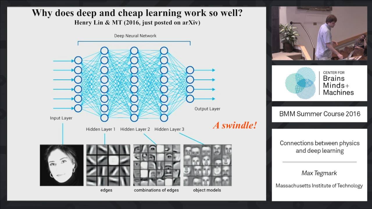
Deep learning succeeds despite combinatorial intractability because the physical universe occupies a tiny, structured subset of functions defined by low-degree polynomial Hamiltonians, locality, and symmetry. (7:40)
Deep architectures provide an exponential efficiency advantage over shallow networks because causal generative hierarchies in nature can be inverted layer-by-layer without losing sufficient statistics. (28:09)
Mutual information across text, Bach's music, genomes, and the 2D critical Ising model decays as a universal power law (~d^-1/2) resulting from tree-like hierarchical generation. (36:03)
Auditing long-range mutual information reveals that standard LSTMs trained on Wikipedia text exhibit a tenfold deficit in long-range semantic retention compared to genuine human language. (48:51)
Detailed notes
## Background
This lecture by MIT professor Max Tegmark was delivered at the Center for Brains, Minds and Machines (MITCBMM) and published on YouTube on August 30, 2016. According to the page metadata and description, the presentation explores the foundational connections between physics and deep learning.
## TL;DR
Tegmark argues that pure mathematics and computer science alone cannot explain why deep learning works so efficiently, asserting that the answer lies in physical laws. Because physical processes are governed by low-degree polynomials, spatial locality, and translation symmetry, reality produces a tiny, highly structured data subset that deep neural networks are uniquely equipped to invert step-by-step. He shows how simple architectures implement multiplication and factorize dense operations, analogizing neural feature abstraction to the renormalization group. Finally, he presents joint research demonstrating that language, music, genomes, and physical systems at phase transitions exhibit power-law mutual information decay, providing a physics-based diagnostic tool to improve recurrent architectures like LSTMs.
## Atmosphere & style
The presentation is intellectually vibrant, playful, and pedagogical, carrying the distinct energy of an interactive academic summer school workshop. Tegmark delivers his arguments with enthusiastic, casual charisma—punctuating rigorous mathematical demonstrations with audience polls, audio excerpts from Bach, and humorous quips about models 'epically sucking' or vortices 'having babies.' The atmosphere feels like a collaborative whiteboard brainstorm across disciplines, shifting from philosophical wonder about the cosmos to grounded engineering diagnostics for artificial intelligence.
## Bulletin
- [07:40](https://www.youtube.com/watch?v=5MdSE-N0bxs&t=460s) Deep learning succeeds despite combinatorial intractability because the physical universe occupies a tiny, structured subset of functions defined by low-degree polynomial Hamiltonians, locality, and symmetry.
- [28:09](https://www.youtube.com/watch?v=5MdSE-N0bxs&t=1689s) Deep architectures provide an exponential efficiency advantage over shallow networks because causal generative hierarchies in nature can be inverted layer-by-layer without losing sufficient statistics.
- [36:03](https://www.youtube.com/watch?v=5MdSE-N0bxs&t=2163s) Mutual information across text, Bach's music, genomes, and the 2D critical Ising model decays as a universal power law (~d^-1/2) resulting from tree-like hierarchical generation.
- [48:51](https://www.youtube.com/watch?v=5MdSE-N0bxs&t=2931s) Auditing long-range mutual information reveals that standard LSTMs trained on Wikipedia text exhibit a tenfold deficit in long-range semantic retention compared to genuine human language.
## Key takeaways
- [00:00](https://www.youtube.com/watch?v=5MdSE-N0bxs&t=0s) Pure mathematics and computer science cannot fully explain deep learning's practical success because generic high-dimensional functions require an impossible exponential number of parameters.
- [04:41](https://www.youtube.com/watch?v=5MdSE-N0bxs&t=281s) Universal approximation theorems guarantee asymptotic expressibility for networks with arbitrary nonlinearities, but practical deep learning is constrained by resource efficiency and learnability.
- [07:40](https://www.youtube.com/watch?v=5MdSE-N0bxs&t=460s) Classifying a 1-megapixel binary image involves 2^1,000,000 potential configurations, yet neural networks perform a combinatorial swindle using only millions or billions of parameters.
- [11:14](https://www.youtube.com/watch?v=5MdSE-N0bxs&t=674s) Bayesian inference maps directly to statistical mechanics by taking negative log-probabilities; the resulting Hamiltonian vector converts into posterior class probabilities via the softmax function.
- [15:22](https://www.youtube.com/watch?v=5MdSE-N0bxs&t=922s) Physical Hamiltonians are remarkably simple, characterized by low polynomial degree (degrees 2 to 4), locality due to relativistic speed-of-light limits, and spatial or temporal symmetry.
- [20:13](https://www.youtube.com/watch?v=5MdSE-N0bxs&t=1213s) Log-probabilities routinely take polynomial forms across science, arising from multivariate Gaussians via the Central Limit Theorem and maximum entropy estimation on statistical moments.
- [22:55](https://www.youtube.com/watch?v=5MdSE-N0bxs&t=1375s) A compact hidden layer with just four nonlinear neurons can implement continuous multiplication via Taylor expansion, allowing neural networks to evaluate arbitrary polynomials.
- [25:48](https://www.youtube.com/watch?v=5MdSE-N0bxs&t=1548s) Biological evolution converged on deep hierarchical neural structures in sensory systems because depth mirrors the sequential, causal structure of the physical environment.
- [28:09](https://www.youtube.com/watch?v=5MdSE-N0bxs&t=1689s) No-flattening theorems prove that hierarchically composed generative processes cannot be compressed into shallow networks without an exponential parameter explosion.
- [31:16](https://www.youtube.com/watch?v=5MdSE-N0bxs&t=1876s) Even purely linear architectures benefit from depth; the Fast Fourier Transform factors a dense O(n^2) operator into log2(n) sparse layers requiring only O(n log n) operations.
- [34:05](https://www.youtube.com/watch?v=5MdSE-N0bxs&t=2045s) The renormalization group in statistical physics provides a theoretical counterpart to deep learning by systematically coarse-graining microscopic noise into macroscopic features.
- [36:03](https://www.youtube.com/watch?v=5MdSE-N0bxs&t=2163s) Human language, Bach's music, chromosome 5, and the critical 2D Ising model exhibit scale-invariant long-range correlations with mutual information decaying as d^-1/2.
- [42:18](https://www.youtube.com/watch?v=5MdSE-N0bxs&t=2538s) Standard 1D Markov chains exhibit exponential correlation decay, whereas top-down hierarchical tree generation produces power laws by composing exponential decay with logarithmic tree distance.
- [46:43](https://www.youtube.com/watch?v=5MdSE-N0bxs&t=2803s) Recursive branching cascades explain power-law phenomena across nature, linking cosmological inflation to Kolmogorov's turbulent vortex fragmentation.
- [48:51](https://www.youtube.com/watch?v=5MdSE-N0bxs&t=2931s) Measuring mutual information decay across distances serves as a diagnostic tool showing that LSTMs hallucinating text underestimate long-range linguistic correlations by roughly a factor of ten.
## Detailed walkthrough
### [00:00](https://www.youtube.com/watch?v=5MdSE-N0bxs&t=0s) Deep Learning at the Nexus of Physics, Neuroscience, and AI
Max Tegmark introduces his talk by focusing on the fruitful overlap between physics and deep learning. Pointing to the center of a Venn diagram uniting physics, neuroscience, and artificial intelligence, he emphasizes that groundbreaking science lives precisely at this convergence. He outlines two distinct examples of problems residing at this intersection, setting out to investigate a foundational question originally posed by Gabriel: why does deep learning work so remarkably well, and how does it accomplish complex tasks so computationally cheaply?
While attendees had already heard accounts throughout the summer school of deep learning’s successes—including theoretical insights from Haim Sompolinsky regarding why deep architectures can outperform shallow ones—Tegmark insists that computer science and pure mathematics cannot provide the whole story. Max Tegmark argues: “I'm going to argue that the full answer to this question cannot be found in mathematics and computer science alone, though. Because part of the answer is actually in physics.”
```mermaid
flowchart TD
accTitle: Intersection of Disciplines
accDescr: Venn diagram style relationship showing Physics, Neuroscience, and AI converging on deep learning questions.
subgraph Disciplines["Foundational Disciplines"]
P["Physics"]
N["Neuroscience"]
AI["Artificial Intelligence"]
end
P --- Center["Core Questions:<br/>Why does deep learning work?<br/>Why is learning efficient?"]
N --- Center
AI --- Center
```
[01:07](https://www.youtube.com/watch?v=5MdSE-N0bxs&t=67s) Feedforward Neural Networks as Function Approximators
Tegmark grounds the discussion by defining a feedforward neural network in elementary mathematical terms: it is simply a function that takes inputs and produces outputs. In computer science and engineering contexts, this means feeding data in and getting data out—whether as raw bits, numeric vectors, or pixel arrays. A feedforward architecture constructs this mapping by iteratively alternating affine transformations (multiplying by a weight matrix and adding bias constants) with simple nonlinearities, such as applying a scalar nonlinear activation function elementwise. Despite the simplicity of this alternating recipe, empirical practice shows that it can tackle astonishingly complex problems.
To illustrate, Tegmark points to familiar real-world breakthroughs. In computer vision, an image containing one million pixels, each defined by red, green, and blue values, can pass through a feedforward network to produce a descriptive natural-language caption, such as "a group of young people playing a game of frisbee." Without retraining, the same network can process a completely different scene and yield an accurate description. Similarly, Google DeepMind’s AlphaGo—which famously defeated world champion Go player Lee Sedol in Seoul—complements reinforcement learning with a deep feedforward value network. This network takes a standard 19-by-19 Go board state, where each intersection is blank, black, or white, and directly computes the winning probability for white.
In everyday applications, these networks typically approximate probability distributions across three major tasks:
- **Prediction:** Forecasting an output variable $y$ given an input $x$ in a stochastic or temporal sequence, such as a smartphone keyboard predicting the next word a user plans to type based on prior keystrokes.
- **Classification:** Inferring the underlying category or identity $x$ given an observed output $y$, such as taking a pixelated portrait under arbitrary lighting conditions and determining which friend’s face is depicted.
- **Unsupervised Density Estimation:** Inferring the true underlying probability distribution directly from unlabelled observations without prior causal assumptions, uncovering latent patterns in raw data.
[04:41](https://www.youtube.com/watch?v=5MdSE-N0bxs&t=281s) Expressibility, Efficiency, and the Combinatorial Swindle
Evaluating how well neural networks approximate functions requires separating performance into three distinct criteria: expressibility (what classes of functions can the architecture represent in principle?), efficiency (how many resources—such as neurons, layers, and synaptic weights—are required?), and learnability (how rapidly and reliably optimization algorithms can discover those optimal parameters). Addressing expressibility, Tegmark notes that stacking successive layers corresponds mathematically to function composition. Consequently, any function space exactly representable by deep networks must be closed under composition.
Tegmark polls the audience on their mathematical background and their familiarity with the classical Stone-Weierstrass theorem, which guarantees that polynomial functions can uniformly approximate any continuous function on a compact domain. Similar universal approximation theorems exist across machine learning literature, showing that neural networks equipped with almost any arbitrary nonlinearity can approximate continuous functions arbitrarily well, provided the network is allowed to grow unbounded.
```mermaid
flowchart LR
accTitle: Neural Network Function Evaluation Dimensions
accDescr: The three core metrics evaluated for neural network approximation: expressibility, efficiency, and learnability.
subgraph Evaluation["Function Approximation Metrics"]
direction TB
E1["Expressibility<br/>(Function classes representable)"]
E2["Efficiency<br/>(Parameters, layers, synapses needed)"]
E3["Learnability<br/>(Convergence speed & optimization)"]
end
E1 --> E2
E2 --> E3
```
- **Compositionally Closed Classes:** Linear mappings, affine maps (linear transformations plus a constant offset), continuous functions, smooth manifolds, polynomials, and piecewise linear functions (formed using rectified linear activation units, or ReLUs).
- **The Stone-Weierstrass Parallel:** Just as polynomials approximate continuous functions arbitrarily closely, networks with arbitrary non-linearities possess universal expressibility given infinite size.
- **The Efficiency Bottleneck:** The critical practical hurdle is not asymptotic expressibility, but efficiency under strict hardware constraints on neurons, depth, and synaptic connections.
[07:40](https://www.youtube.com/watch?v=5MdSE-N0bxs&t=460s) The Mathematical Impossibility and the Role of Physics
When shifting from asymptotic expressibility to resource efficiency, Tegmark highlights a profound mathematical paradox: from a purely combinatorial perspective, deep learning ought to fail completely. Max Tegmark explains: “Because if you start to think about this question of in the red box here, after a while, you realize that it's kind of shocking that deep learning works at all, that it doesn't epically suck.”
To demonstrate why, he presents a simple classification problem: distinguishing between two friends, Gabriel and Maya, from a 1,000-by-1,000 black-and-white grid. An image of this resolution contains $10^6$ binary pixels, yielding $2^{1,000,000}$ possible visual inputs. To store a generic, arbitrary mathematical function assigning a classification probability to every individual configuration, one would need to specify $2^{1,000,000}$ independent parameters. For comparison, the entire observable universe contains roughly $10^{89}$ elementary particles. Mapping generic high-dimensional inputs should therefore be utterly impossible.
Yet deep learning executes a dramatic "combinatorial swindle," substituting exponential parameter scaling with mild polynomial multiplication. A network with an input layer of one million units and a modest stack of layers—whether three or two hundred—requires only on the order of millions or billions of parameters, nowhere near $2^{1,000,000}$. Pure mathematics states that the fraction of high-dimensional functions representable by such tiny parameter sets is of measure zero. Tegmark concludes that the feasibility of deep learning cannot stem from mathematics alone. Instead, the answer lies in physics: the physical universe does not produce generic states. A mathematically typical 1-megapixel image is indistinguishable from pure white noise, a fact proven by Émile Borel over a century ago in his analysis of normal numbers, whose binary expansions pass every statistical test of randomness. Real-world images of friends like Gabriel occupy an infinitesimal, highly structured subset of reality shaped by physical laws.
[11:14](https://www.youtube.com/watch?v=5MdSE-N0bxs&t=674s) Bayes’ Theorem, the Boltzmann Distribution, and Softmax
Max Tegmark sets out to investigate the special class of functions that neural networks excel at computing, comparing them to the functions generated by physics and real-world imagery such as drawings and cartoons. He argues that the two classes are essentially identical, providing the fundamental reason deep learning performs so well. To illustrate the connection, he considers an image classification task: deciding whether an image depicts Gabriel or his wife Maya. Beginning with a prior probability distribution over the identity $x \in \{\text{Maya}, \text{Gabriel}\}$ and a generative model of what the image looks like given $x$, one can apply Bayes' theorem to find the posterior probability of identity given the observed data.
Tegmark translates Bayes' theorem into the language of physics by taking the negative logarithm of the probabilities. Through this transformation, products of conditional probabilities convert into sums, directly mirroring the Boltzmann distribution of statistical mechanics. In physics, high-dimensional probability distributions are typically tractable because variables exhibit conditional independence, allowing the total energy—the Hamiltonian—to decompose into a sum of distinct energy contributions. Looking at the exact same mathematics through a machine learning lens reveals that this normalized exponent of negative log-probabilities is precisely the softmax function: exponentiating the vector entries and rescaling them so they sum to one. Defining the vector $H$ with entries representing the negative log-probability (surprisal) for Gabriel and Maya, Tegmark demonstrates that optimal Bayesian inference requires only estimating the Hamiltonian before feeding it into a terminal softmax layer. As Tegmark states: “So what this is saying in plain English is that if I can somehow build the neural network that will really, really accurately approximate the Hamiltonian, or the log probability in other words, for these pictures of Maya or pictures of Gabriel or whatever else it is I have, then I'm done.”
```mermaid
flowchart LR
accTitle: Bayesian Inference via Softmax
accDescr: Pipeline mapping raw input data through a Hamiltonian network to class probabilities using softmax.
subgraph InputStage["Observation"]
Img["Input Data / Image"]
end
subgraph EnergyStage["Feature Extraction"]
HNet["Neural Network: Compute H(x)"]
end
subgraph OutputStage["Bayesian Posterior"]
SM["Softmax Layer"]
Out["P(Maya | Image), P(Gabriel | Image)"]
end
Img --> HNet
HNet --> SM
SM --> Out
```
[15:22](https://www.youtube.com/watch?v=5MdSE-N0bxs&t=922s) Why Physical Hamiltonians are Simple: Low Degree, Locality, and Symmetry
Tegmark poses the question of whether there is any valid reason to expect the Hamiltonian of the physical world to be simple to calculate. In physics, formulating a system's Hamiltonian—the function specifying energy based on particle positions and internal parts—is a primary pursuit. Remarkably, empirical physics shows that the Hamiltonian of our universe is not an arbitrary function. At CERN, the Standard Model of particle physics used to evaluate the Higgs boson relies on a polynomial Hamiltonian of remarkably low degree: degree 4, where the quartic power originates from the Higgs particle, while remaining components are quadratic or cubic.
To demonstrate how constraints reduce complexity, Tegmark walks through a concrete one-dimensional audio modeling problem where a microphone records ten sequential air pressure measurements, $x_1, x_2, \dots, x_{10}$, to identify a speaker's voice:
- **Arbitrary general function**: Specifying an arbitrary continuous function of 10 variables requires infinitely many parameters.
- **General polynomial (quadratic)**: Restricting the Hamiltonian to a quadratic polynomial allows each variable to interact with every other variable, reducing the parameter count to 66 pairs.
- **Locality**: Physical interactions do not propagate instantaneously; by the speed of light, forces act locally. Limiting coupling solely to nearest neighbors and self-interactions drops the parameter count to 20.
- **Symmetry (Invariance)**: The laws of physics are invariant across space and time. Because the correlation between voice air pressures separated by a tenth of a second does not depend on the absolute time of recording, coupling between $x_1$ and $x_2$ matches the coupling between $x_7$ and $x_8$. Enforcing translation symmetry collapses the entire model down to just two parameters: one for nearest-neighbor coupling and one for self-interaction.
Beyond the fundamental Standard Model, effective and approximate physical descriptions exhibit this same structure. The Navier-Stokes equations governing fluid dynamics—useful for modeling ocean water on a beach—possess degree-3 polynomial Hamiltonians characterized by locality and symmetry. Maxwell's equations for electromagnetism are even simpler quadratic polynomials. Tegmark stresses that almost every approximate equation written in physics is a highly sparse, low-degree polynomial.
[20:13](https://www.youtube.com/watch?v=5MdSE-N0bxs&t=1213s) Log-Probabilities as Polynomials in Physics and Machine Learning
Responding to an audience question asking why the negative logarithm of a probability distribution is labeled a Hamiltonian, Tegmark clarifies that in thermal equilibrium, physical probabilities routinely appear as $e^{-E / k_B T}$. However, the convenience of negative log-probabilities extends well beyond pure physical equilibrium. In many complex systems where numerous independent phenomena combine linearly, the Central Limit Theorem dictates that the resulting distribution is a multivariate Gaussian. Because a Gaussian distribution takes the form of $e^{-\text{quadratic}}$, its negative logarithm is strictly a quadratic polynomial.
Similarly, in machine learning, maximum entropy estimation selects the least biased distribution matching measured statistical moments (such as second, third, or fourth moments). Mathematically, maximum entropy distributions conditioned on fixed moments are guaranteed to take the form of an exponential of a polynomial, ensuring the negative log-probability remains a low-degree polynomial. Tegmark points out that whether analyzing photographs of galaxies generated by astrophysical processes or standard machine learning datasets, data distributions fundamentally originate from sparse polynomial Hamiltonians. As Tegmark summarizes: “The log probability is very often the polynomial. And if it is a polynomial, then you can totally trust the classification problem if your own neural network is good at approximating polynomials.” He concludes the segment by noting that polynomials are not merely possible to approximate, but can be computed exactly by simple neural network architectures.
[22:55](https://www.youtube.com/watch?v=5MdSE-N0bxs&t=1375s) Implementing Multiplication with Hidden Neurons
While universal approximation theorems demonstrate what can be accomplished given an arbitrarily large neural network, Max Tegmark illustrates that an extremely compact architecture—just four neurons in a hidden layer—can already implement the multiplication of two continuous numbers. In the schematic he presents, circular summation nodes add incoming signals, square nodes apply a nonlinear activation function $\sigma$, and directed edges scale inputs by weights such as $\lambda$ and $\mu$. For any activation function that is not purely linear, shifting it with a bias term guarantees a non-zero second derivative at the origin. Taking the Taylor expansion of this arrangement shows that combining four specific input configurations yields the exact product of the two inputs plus an unavoidable fourth-order error term. By scaling down the input weights with a small factor $\lambda$, the error term becomes negligible, after which the output can simply be scaled back up to produce a clean multiplication gate.
```mermaid
flowchart LR
accTitle: Four-Neuron Multiplication Gate
accDescr: Flowchart showing two input numbers routed through four nonlinear hidden neurons and summed to compute their product.
subgraph Inputs["Inputs"]
U["Input u"]
V["Input v"]
end
subgraph Hidden["Hidden Layer (scaled by small λ)"]
H1["σ(λ(u + v))"]
H2["σ(λ(u - v))"]
H3["σ(λ(-u + v))"]
H4["σ(λ(-u - v))"]
end
subgraph Output["Summation & Rescaling"]
S["Sum & Rescale (1/λ²)"]
P["Product: u · v"]
end
U --> H1 & H2 & H3 & H4
V --> H1 & H2 & H3 & H4
H1 --> S
H2 --> S
H3 --> S
H4 --> S
S --> P
```
Because addition requires only a single trivial layer in a neural network, coupling addition with this multiplication gate enables the network to express arbitrary polynomials by stacking layers. When working with binary inputs rather than continuous variables, computing multiplication becomes even simpler. While multiplying multiple continuous numbers pairwise requires adding layers for each additional factor, multiplying arbitrary binary bits requires only a single hidden neuron. The product of binary digits can equal 1 if and only if every single bit is 1. If there are three bits, their sum must equal 3. By feeding the sum into a standard sigmoid activation function with a threshold set between 2 and 3, a single neuron easily determines whether all bits are active.
- “And once you can multiply numbers, of course, addition comes for free in neural network.”
- A shifted nonlinear activation function with $\sigma''(0) \neq 0$ eliminates lower-order interference, leaving only the product and a fourth-order residue $O(\lambda^4)$.
- For binary multiplication across $k$ inputs, the hidden neuron evaluates $\sum_{i=1}^k x_i$ and thresholds the sum at $k$ versus $k-1$.
[25:48](https://www.youtube.com/watch?v=5MdSE-N0bxs&t=1548s) Why the Physics of the Real World Matches Neural Networks
Tegmark highlights a fundamental alignment between physics and machine learning: the universe does not generate arbitrarily random probability distributions for images, sounds, or other physical phenomena. Instead, the natural world produces an extraordinarily narrow, structured subset of possible data distributions. Correspondingly, while neural networks are mathematically incapable of approximating the vast majority of generic mathematical functions, they happen to excel at modeling the specific subset generated by physical laws. Tegmark contends that this alignment is no mere accident, noting that biological evolution recognized and exploited these physical regularities long before human engineers:
> “We are very excited to be humans because we invented deep learning. But of course, evolution scooped us.”
The primate visual cortex and other well-understood brain structures rely heavily on hierarchical, deep processing because it tapped directly into the structured regularities of the physical environment. Tegmark suggests that analyzing the mathematical structures produced by physical processes—and human activities patterned on physics, such as drawing and handwriting—provides a concrete roadmap for designing and optimizing artificial neural architectures. This connects directly to the insights shared by Haim Sompolinsky regarding "cheap learning": neural networks succeed not merely because they approximate functions with millions of parameters instead of a googolplex, but because their depth provides an inductive bias that reflects how reality unfolds.
- “And neural networks are very, very good at approximating almost no functions. But they're really, really good at approximating this very special kind that nature feeds us.”
- Evolution converged on deep hierarchical networks in sensory systems because they mirror the physical regularities of the external world.
- "Cheap learning" refers to achieving high predictive accuracy with a tiny parameter footprint relative to the theoretical worst-case dimensionality.
[28:09](https://www.youtube.com/watch?v=5MdSE-N0bxs&t=1689s) Generative Hierarchies and No-Flattening Theorems
To explain why deep networks outperform shallow ones, Tegmark examines how physical processes generate data. In nature, data generation is inherently sequential: one event happens, which causes the next, and so on down a causal chain. The same structure appears in computer graphics; rendering a ray-traced image of a cat requires first selecting the animal class, choosing solid-modeling geometric parameters, and finally running ray-tracing rendering calculations. In their paper, Tegmark and his collaborator proved that when data originates from such a hierarchical generative process, there is an optimal mathematical inversion that reconstructs the initial state without losing information beyond the unavoidable entropy added by noise:
> “And what you find is, not surprisingly at all, that the best way of analyzing data is to just undo the complications that nature made for you one step at a time.”
This stepwise reversal links directly to sufficient statistics, the branch of statistics dedicated to identifying estimators that capture all informative content from samples. Because individual physical transitions are local and relatively simple, neural networks can model and invert each step with high efficiency. Reversing a generative process with twenty simple physical steps naturally yields a twenty-layer neural network.
```mermaid
flowchart TD
accTitle: Generative Process and Inverse Deep Network
accDescr: Diagram contrasting the forward generative steps of nature with the inverse layer-by-layer reconstruction performed by a deep neural network.
subgraph Forward["Physical Generative Process"]
direction TB
G0["Scene Intent: Pick Cat"] --> G1["Geometric Modeling"]
G1 --> G2["Lighting & Ray-Tracing"]
G2 --> G3["Raw Pixel Observation"]
end
subgraph Inverse["Deep Neural Network Inversion"]
direction BT
L0["Layer 1: Edge & Feature Detection"] --> L1["Layer 2: Shape & Parts Extraction"]
L1 --> L2["Layer 3: Object Classification (Cat)"]
end
G3 -.->|"Feed into network"| L0
```
The superiority of deep architectures implies that these layered graphs cannot be compressed into shallow networks without severe performance penalties. Tegmark calls the mathematical formalization of this constraint "no-flattening theorems." If a five-layer network achieves an objective using a modest budget of neurons and synaptic weights, a no-flattening theorem proves that achieving equivalent accuracy with fewer layers requires an exponential explosion of parameters. He points to research by Tommy Poggio and collaborators demonstrating that composing functions hierarchically creates computational efficiencies that cannot be flattened into shallow networks without requiring exponentially more resources.
- “Tommy Poggio, with collaborators for example, has written a series of beautiful papers showing that if you have a hierarchical process where you compose functions, there are many situations where you cannot flatten them without having to have exponentially more resources.”
- Generative hierarchies in physics lose information monotonically due to noise, but stepwise inversion preserves all available sufficient statistics.
- A twenty-step generative mechanism maps naturally onto a twenty-layer deep network rather than a single collapsed layer.
[31:16](https://www.youtube.com/watch?v=5MdSE-N0bxs&t=1876s) Why Deep is Better Even in Linear Networks: FFT and Renormalization
To demonstrate that depth advantages do not depend entirely on nonlinearities, Tegmark introduces a counterintuitive case: deep, entirely linear networks. While a critic might dismiss linear networks because any sequence of matrix multiplications can mathematically be collapsed into a single matrix product, Tegmark points out that flattening a linear network can dramatically impair computational efficiency. Compressing the layers preserves the input-output function and may reduce intermediate neuron counts, but it often causes an explosion in the number of required non-zero synaptic weights and operations.
The classic demonstration of this principle is the Fast Fourier Transform (FFT). Applying a discrete Fourier transform directly to a vector of $n = 1{,}024$ numbers using a single flat layer requires multiplying by a dense $1{,}024 \times 1{,}024$ matrix of complex numbers, demanding roughly $n^2 \approx 10^6$ operations. The FFT algorithm instead factors that dense operator into $\log_2(1{,}024) = 10$ sparse matrices, each containing only about $2n$ non-zero parameters representing simple pairwise sums and differences:
> “So if you have a nice deep network with 10 layers that does the FFT, if you flatten it, now it's going to be n squared. Almost 1,000 times slower. 100 times slower. That sucked. So you see even for linear networks sometimes deep is much better.”
Tegmark notes that this factorized sparsity appears throughout applied mathematics, including discrete wavelet transforms and fast matrix multiplication algorithms that drop arithmetic complexity from naive $O(n^3)$ scaling down to $O(n^{2.4})$. He concludes by tying this phenomenon directly back to theoretical physics: the renormalization group. In physics, renormalization provides a systematic mathematical machinery for isolating the macroscopic properties that observers care about while progressively averaging out and discarding irrelevant microscopic degrees of freedom. This physical coarse-graining across scales operates as an exact physical counterpart to layer-by-layer data abstraction in deep learning.
- “And finally this has a lot to do with physics... the whole business with renormalization in physics, which is the process by which we extract information we care about while ignoring all the things we don't care about is very analogous to this process of analyzing data and deep learning.”
- Flattening an FFT network replaces $n \log_2 n$ operations with $n^2$, illustrating that depth provides parameter efficiency independent of non-linear activations.
- Renormalization in statistical physics serves as a formal analogue for feature pooling and abstraction across successive layers of deep networks.
[34:53](https://www.youtube.com/watch?v=5MdSE-N0bxs&t=2093s) Understanding Deep Learning to Make It Robust and Efficient
Reflecting on how neural networks distill features and discard noise, Max Tegmark explains that bridging physics, artificial intelligence, and neuroscience helps uncover the underlying reasons why deep learning performs so remarkably well. Gaining this theoretical foundation is not just an academic exercise; understanding the mechanisms of deep learning provides concrete pathways to improve it. Tegmark highlights two major objectives: improving resource efficiency so models learn faster and approximate functions with fewer computational resources, and improving robustness so systems reliably do what humans intend rather than falling prey to catastrophic failures.
As an illustration of the brittleness in current systems, Tegmark refers to adversarial training examples where tiny, imperceptible perturbations lead neural networks to make absurd classification errors. “And my hope is that the more we can understand why deep learning works so well, the greater the chances are that we can make it work even better also,” Tegmark states, emphasizing that better understanding ensures a network “doesn't get fooled into thinking that a person is a starfish, for those of you who heard of this famous adversarial training example.”
- **Efficiency goals**: Accelerating learning rates and approximating complex functions using fewer parameters and less computational power.
- **Robustness goals**: Preventing adversarial vulnerability and ensuring networks behave predictably in real-world environments.
---
[36:03](https://www.youtube.com/watch?v=5MdSE-N0bxs&t=2163s) The Mystery of Power Laws Across Music, Language, Genomes, and Magnets
Tegmark transitions to another striking link between physics and deep learning: phase transitions and critical phenomena. He presents research conducted collaboratively with Harvard student Henry Lin at MIT, displaying an unexpected plot where radically different domains share identical scaling behavior on the exact same axes. The plot compares French text, English text, Johann Sebastian Bach's music, the human genome (specifically chromosome 5), and a simulated physical system—the 2D Ising model of a magnet right at its demagnetization phase transition.
```mermaid
flowchart TD
accTitle: "Information Decay Across Diverse Systems"
accDescr: "Comparison of Markovian exponential decay versus hierarchical power-law decay in language, music, genomes, and physics."
subgraph CriticalProcess["Scale-Invariant Systems"]
C["Hierarchical Tree Generation"] --> D["Distance Between Nodes = Logarithmic"]
D -->|"Exp(-Log(t))"| E["Power-Law Mutual Information Decay (~ d^-1/2)"]
end
E -.-> F["English & French Text"]
E -.-> G["Bach Violin Music"]
E -.-> H["Human Chromosome 5"]
E -.-> I["2D Ising Model at Critical Temp"]
```
Because correlation functions require multiplying numerical values—which works for magnetic spins but fails for discrete symbols like musical notes or letters—Lin and Tegmark generalized the metric using mutual information. They asked: if an observer hears a tone in a Bach piece, how many bits of information does that tone provide about a note occurring ten or more steps into the future? In all examined datasets, mutual information decays not exponentially, but as a power law with a slope of roughly minus one-half ($d^{-1/2}$). Tegmark admits their utter astonishment at the data: “So we were very shocked, honestly, when we looked at all these curves.”
- **Generalized metric**: Mutual information in bits replaces standard correlation functions for non-numerical categorical sequences.
- **Slope of decay**: All systems exhibited a power-law falloff of mutual information roughly proportional to $d^{-1/2}$.
- **Analyzed data**: Bach compositions, English text, French text, human chromosome 5, and the 2D Ising model.
---
[38:20](https://www.youtube.com/watch?v=5MdSE-N0bxs&t=2300s) Phase Transitions and Long-Range Correlations in the Ising Model
To develop intuition for this phenomenon, Tegmark demonstrates the physics of a two-dimensional Ising model, consisting of a 2D grid of microscopic magnetic spins pointing either up or down. At high temperatures, thermal fluctuations dominate, causing spins to point randomly in uncorrelated directions. As the grid is cooled, neighboring spins attempt to align. At a specific critical temperature—analogous to liquid water abruptly freezing into structured ice—the system undergoes a second-order phase transition. Exactly at this critical point, mutual information between spins falls off as a power law, scaling as the inverse square root of distance.
At any temperature away from this critical point, or in any conventional Markov process where the next state depends solely on the immediate predecessor, correlations die off exponentially because distant points remain completely agnostic of each other. The data, however, revealed that music, human language, and genetic sequences exhibit scale-invariant, long-range correlations that mirror critical physical systems. Playing an excerpt of Bach's violin music performed by Hilary Hahn (recognized by audience member Gabriel), Tegmark notes that music contains short-term predictive structure alongside themes and motifs that recur over vast temporal distances. Similarly, English displays structure across multiple hierarchical tiers: letters combine into phonemes, phonemes into words (such as anticipating the letter "u" after seeing "o-p-o-s-s" to spell "opossum"), words into sentences, sentences into paragraphs, and paragraphs into high-level ideas.
“At exactly this critical temperature you can calculate that the information they have about the neighbors falls off like this one over the square of the distance power law,” Tegmark explains, noting that away from criticality, “what typically happens is that these correlations always die off exponentially.”
- **Markovian limitation**: Traditional Markov chains discard memory such that mutual information decays strictly exponentially.
- **Critical phenomena**: Only at the critical transition temperature do spatial correlations persist across macroscopic distances in the 2D Ising model.
- **Hierarchical nesting**: Text and music exhibit multi-scale correlation hierarchies, from local adjacent tokens up to overarching themes.
---
[42:18](https://www.youtube.com/watch?v=5MdSE-N0bxs&t=2538s) Hierarchical Generative Trees and the Emergence of Power Laws
The presence of power-law scaling in language, music, and DNA presented a severe theoretical paradox. In statistical physics, a rigorous theorem proves that phase transitions with power-law correlations cannot exist in purely one-dimensional systems; they require two, three, or more spatial dimensions. Yet text, musical audio, and DNA are strictly one-dimensional sequences. Lin and Tegmark realized the resolution lies in hidden dimensional structures: recursive, hierarchical generation.
When humans write a report, prepare a presentation for a workshop, or compose a symphony, they do not generate sequences sequentially from left to right like a linear Markov process. Instead, generation operates as a top-down branching tree—analogous to Noam Chomsky's universal grammar and phrase-structure trees. A presenter starts with an overarching thesis, partitions it into key ideas, breaks those into individual slides, and finally writes specific bullet points and words. If a process retains 90% of its information per step, a sequential chain loses $(0.9)^t$ exponentially. But in a tree structure, two sequence elements separated by linear time $t$ share a common ancestor whose path distance through the hierarchy scales only logarithmically with time ($\log t$).
When an exponential decay rate is evaluated over a tree distance that grows logarithmically, the exponential and logarithmic functions compose to yield an exact power law: $\exp(-\alpha \log t) = t^{-\alpha}$. Tegmark links this mathematical mechanism directly back to cosmology: “Interestingly in physics if you look at power laws, they're always, as far as I can tell, also created by almost the same kind of thing.” He cites MIT colleague Alan Guth's theory of cosmic inflation, where the exponential doubling of space similarly produces scale-invariant power-law correlations in the clumpiness of cosmic matter across the universe.
- **Physics paradox**: 1D physical chains cannot support critical phase transitions, implying 1D data sequences must possess an underlying higher-dimensional tree topology.
- **Logarithmic path length**: In a branching tree with branching factor 2, the network distance to the lowest common ancestor scales as $\log_2(t)$.
- **Mathematical cancellation**: $\exp(-c \cdot \log t) \propto t^{-c}$, directly transforming exponential information decay across tree depth into power-law spatial correlations.
- **Cosmological parallel**: Alan Guth's inflationary expansion doubles space repeatedly, yielding a power-law correlation spectrum for cosmic matter distribution.
[46:43](https://www.youtube.com/watch?v=5MdSE-N0bxs&t=2803s) Recursive Cascades, Kolmogorov Turbulence, and Power Laws
Max Tegmark explains the physical mechanism behind the emergence of power laws, drawing a direct parallel between cosmic inflation and fluid turbulence. In cosmology, a small patch of space begins with random fluctuations, doubles in size, and then each subregion repeats the exact same fluctuation-generating process, passing its ancestral perturbations down to subsequent generations in a recursive branching tree. A nearly identical cascade occurs in fluid dynamics: Andrei Kolmogorov showed that water flowing from a tap or cascading down a waterfall exhibits power-law correlations across spatial velocities because large vortices continually fragment into smaller vortices. Tegmark describes this vivid mental picture:
> “Well, Kolmogorov realized that you get these little vortices or eddies and they tend to have babies.”
These larger eddies generate offspring approximately half their size, which in turn spawn even smaller child vortices all the way down the scale. Because nature relies on this self-similar, fractal doubling mechanism across multiple domains, physical observables repeatedly organize into clean power-law distributions.
```mermaid
flowchart TD
accTitle: Hierarchical Cascade Process
accDescr: Diagram illustrating how large scale structures recursively spawn smaller child structures across scales.
subgraph MacroScale ["Large Scale"]
A["Parent Entity<br/>(Space patch / Large eddy)"]
end
A --> B1
A --> B2
B1 --> C1
B1 --> C2
B2 --> C3
B2 --> C4
```
[47:54](https://www.youtube.com/watch?v=5MdSE-N0bxs&t=2874s) Hierarchical LSTMs and Long-Range Information Curves
Tegmark bridges these recursive cascades directly to modern deep learning architectures by querying the audience about recurrent neural networks. He singles out Long Short-Term Memory (LSTM) networks, noting that they have become a major commercial workhorse across the tech industry. By arranging recurrent units in a layered hierarchy, one can construct an architecture that mimics physical cascades: each higher layer retains information for twice as long as the layer beneath it. This structure naturally mirrors the multi-scale temporal and spatial correlations found in nature.
Tegmark argues that tracing the decay of mutual information across distances—measuring how much information an early point in a sequence retains about points farther down the road and plotting that correlation curve—is not just an abstract mathematical exercise. Instead, it serves as a powerful practical metric for machine learning practitioners seeking to evaluate and optimize neural networks for real-world sequential tasks.
- LSTMs serve as an architectural tool to capture multi-scale temporal hierarchies.
- Stacking layers with progressively doubled retention timescales naturally replicates power-law memory curves.
[48:51](https://www.youtube.com/watch?v=5MdSE-N0bxs&t=2931s) Diagnosing Text Prediction and the Hutter Prize
Applying this diagnostic framework to sequential tasks like text auto-correction and data compression reveals clear limitations in current systems. Tegmark explains that standard supervised training teaches a network to guess the immediate next token, rewarding correct hits and penalizing misses. Yet achieving a high raw accuracy rate—such as 90% next-token accuracy or a low Kullback–Leibler divergence score—fails to tell an engineer whether their architecture has genuinely saturated the statistical structure of human language.
He references the famous Hutter Prize, an open benchmark competition dedicated to compressing the text of Wikipedia as densely as possible. While the leading compression mark stood at around 16%, engineers had no principled benchmark to prove whether English text could theoretically be compressed further or if current models had hit an intrinsic wall. Tegmark emphasizes this uncertainty:
> “If you only know that you accomplished 16% with your neural network and you trained really hard, there's no real way of knowing.”
The correlation curve provides the missing diagnosis. While traditional Markov processes fail miserably on language, an LSTM trained on Wikipedia text is capable of competitive compression performance. However, when that trained LSTM is allowed to run autonomously and hallucinate future text, an empirical audit reveals a major blind spot: the network accurately predicts immediate adjacent characters, but its long-range mutual information curve decays far too quickly, falling short of real English text by roughly a factor of ten.
- Supervised next-character loss metrics conceal failures to model macroscopic, long-range context.
- The Hutter Prize record of approximately 16% Wikipedia compression leaves open the question of whether language has reached its fundamental entropy limit.
- Generative text hallucinated by LSTMs reveals a 10× deficit in capturing long-range semantic correlations compared to actual Wikipedia text.
[51:05](https://www.youtube.com/watch?v=5MdSE-N0bxs&t=3065s) The Interface of Physics, Neuroscience, and AI
Tegmark concludes by summarizing the broader philosophical and practical advantages of cross-pollinating disciplines. Treating neural networks through the analytical lens of physics offers more than mathematical curiosity; it provides concrete diagnostic tools that help engineers discover why empirical models hit plateaus and how they can be systematically redesigned.
He invites the audience to explore the rich intersections among physics, computational neuroscience, and artificial intelligence, asserting that the most exciting research questions still lie unresolved at this shared boundary:
> “I feel that there's a lot of wonderful stuff left to do.”
## Notable quotes
> [25:48](https://www.youtube.com/watch?v=5MdSE-N0bxs&t=1548s) Neural networks are very, very good at approximating almost no functions. But they're really, really good at approximating this very special kind that nature feeds us. — Max Tegmark
> [25:48](https://www.youtube.com/watch?v=5MdSE-N0bxs&t=1548s) We are very excited to be humans because we invented deep learning. But of course, evolution scooped us. — Max Tegmark
> [28:09](https://www.youtube.com/watch?v=5MdSE-N0bxs&t=1689s) The best way of analyzing data is to just undo the complications that nature made for you one step at a time. — Max Tegmark
## Mentioned
Max Tegmark, Gabriel, Haim Sompolinsky, AlphaGo, Google DeepMind, Lee Sedol, Stone-Weierstrass theorem, Émile Borel, Maya, CERN, Higgs boson, Navier-Stokes equations, Maxwell's equations, Tommy Poggio, Fast Fourier Transform, Henry Lin, Johann Sebastian Bach, Hilary Hahn, Noam Chomsky, Alan Guth, Andrei Kolmogorov, Hutter Prize, Wikipedia
Physicist Max Tegmark argues that the unexpected success and resource efficiency of deep learning cannot be explained by mathematics and computer science alone, but fundamentally stem from the structured laws and hierarchical generative mechanisms of the physical universe.
The Combinatorial Swindle and Physical Constraints (7:40)
From a purely mathematical standpoint, general function approximation across high-dimensional spaces should fail combinatorially. For example, distinguishing between two faces on a 1,000-by-1,000 black-and-white grid requires selecting among $2^{1,000,000}$ possible states, demanding vastly more parameters than the approximately $10^{89}$ elementary particles in the observable universe. Deep neural networks bypass this combinatorial bottleneck by substituting exponential parameter scaling with modest polynomial parameter budgets.
Physical Hamiltonians, Low Degrees, and Symmetries (15:22)
Tegmark explains that optimal Bayesian inference reduces to computing an energy function, or Hamiltonian, before a terminal softmax layer converts negative log-probabilities into classification probabilities. Crucially, physical systems are governed by Hamiltonians that are not arbitrary high-dimensional functions, but sparse, low-degree polynomials. For instance, the Standard Model of particle physics has a maximum degree of four, fluid dynamics via the Navier-Stokes equations is degree-three, and electromagnetism is quadratic. Combined with physical locality—constrained by the speed of light—and spatial or temporal symmetries, the parameter count needed to describe physical phenomena collapses from infinity to a manageable handful. Because neural networks can easily compute addition and multiplication using simple hidden-layer nonlinearities, they natively reflect and capture these sparse polynomial structures.
Hierarchical Inversion and Depth Efficiency (28:09)
Physical data generation is fundamentally sequential and hierarchical, where one causal transition leads to another, as seen in step-by-step computer graphics rendering. Tegmark points to "no-flattening theorems" developed with collaborators and by Tommy Poggio, which prove that stepwise hierarchical processes cannot be collapsed into shallow architectures without an exponential explosion in parameter requirements. Stepwise inversion naturally maps a multi-step physical process onto a deep network that extracts sufficient statistics at each layer while progressively discarding irrelevant microscopic variations, mirroring the renormalization group in statistical physics. This depth advantage holds even in entirely linear operations; for instance, the Fast Fourier Transform uses a 10-layer factorized architecture with $O(n \log n)$ operations, whereas flattening it into a single layer demands an $O(n^2)$ dense matrix calculation that is up to 1,000 times slower.
Power-Law Correlations and Hierarchical Generation (36:03)
Investigating empirical data across English text, French text, Bach's violin music, human chromosome 5, and the 2D Ising model at its critical phase transition, Tegmark and Henry Lin observed that mutual information decays as a power law with a slope near $d^{-1/2}$, rather than decaying exponentially like a standard Markov chain. Because physical theorems forbid critical phase transitions in strictly one-dimensional systems, Tegmark explains that 1D text and genetic sequences must originate from top-down branching tree structures, similar to Chomskyan phrase structures, cosmic inflation, or Kolmogorov turbulence cascades. In a branching tree, linear separation $t$ corresponds to a path distance through a common ancestor of order $\log t$, causing exponential information loss $\exp(-\alpha \log t)$ to cancel cleanly into scale-invariant power-law decay $t^{-\alpha}$.
Diagnosing Machine Learning Deficits with Physics (47:54)
Tegmark notes that while deep networks excel on short-range token prediction, tracking physical correlation curves provides a diagnostic tool to expose deeper algorithmic blind spots. For instance, Long Short-Term Memory networks (LSTMs) trained on Wikipedia compress text effectively, achieving competitive marks in the Hutter Prize, but generative text hallucinated by these models reveals that long-range mutual information drops off roughly ten times faster than in authentic English text. Applying physical metrics like mutual information decay exposes these hidden contextual failures that conventional next-step loss functions routinely mask.
Tegmark concludes that grounding artificial intelligence in the mathematical principles of physics and computational neuroscience provides a practical foundation to move beyond empirical trial and error. Deepening this theoretical connection is critical for engineering architectures that avoid adversarial vulnerabilities, learn with greater parameter efficiency, and capture multi-scale real-world structures.
## Background
该视频由麻省理工学院大脑、心智与机器中心(MITCBMM)于 2016 年 8 月 30 日在 YouTube 平台发布。视频内容为麻省理工学院物理学家马克斯·泰格马克(Max Tegmark)题为《物理学与深度学习的联系》(Connections between physics and deep learning)的主题演讲。
## TL;DR
马克斯·泰格马克指出,深度学习之所以能避免“维度灾难”而高效运作,本质答案不在纯数学或计算机科学中,而深植于物理学法则。真实世界的物理系统由低阶多项式、定域性、对称性及分层因果生成过程所主导,这恰好完美契合了深度神经网络交替应用线性变换与非线性激活的函数逼近优势。泰格马克通过四神经元乘法门、快速傅里叶变换(FFT)的深层稀疏分解、以及“不可展平定理”,论证了为何深层架构显著优于浅层结构。最后,他揭示了语言、音乐、基因与二维伊辛模型在相变临界点处共享的幂律长程关联,并展示了如何利用物理学的互信息关联曲线来有效诊断与优化神经网络的长程建模能力。
## Atmosphere & style
整场演讲充满智识碰撞的激情与幽默风趣的学者风范,泰格马克以通俗生动的比喻解构深奥的理论物理与机器学习数学,现场互动频繁且引人入胜。他的叙述节奏明快,从“深度学习本该烂得史诗级彻底”的惊人悖论开场,一路层层拆解、峰回路转,最终将听众引向物理宇宙生成规律与智能本质统一的壮丽图景。整场分享洋溢着跨学科探索的纯粹好奇心与思想解放感,令听众既能领会严谨数学论证的精妙,又能真切感受到前沿科学交汇处的磅礴魅力。
## Bulletin
- [07:20](https://www.youtube.com/watch?v=5MdSE-N0bxs&t=440s) Max Tegmark 指出,从纯数学角度来看,神经网络能逼近的函数在所有可能函数中测度为零;深度学习之所以未陷入“指数级爆炸”的组合灾难,根本原因在于物理世界生成的真实数据受到极低阶多项式、定域性与对称性等物理定律的严苛约束。
- [11:14](https://www.youtube.com/watch?v=5MdSE-N0bxs&t=674s) 图像分类与概率建模中的 Softmax 函数和贝叶斯对数似然,在物理学中严格对应于微观能量分布的玻尔兹曼分布与哈密顿量,而神经网络仅需 4 个隐藏神经元即可基于泰勒级数精确构造出乘法门以逼近多项式。
- [31:16](https://www.youtube.com/watch?v=5MdSE-N0bxs&t=1876s) 即便是纯线性网络,“深层”也能带来颠覆性优势:例如快速傅里叶变换(FFT)通过 10 层稀疏分解将计算复杂度从单层展平矩阵的 O(n²) 压缩至 O(n log n),强行展平为浅层网络反而会导致参数量和计算开销急剧暴增。
- [36:03](https://www.youtube.com/watch?v=5MdSE-N0bxs&t=2163s) 人类语言、巴赫音乐、基因组与二维伊辛模型在相变临界态下均表现出斜率约 -0.5 的互信息幂律衰减;借助物理两点关联函数诊断发现,顶级 LSTM 即使单步预测准确率极高,其长程关联度仍比真实文本低一个数量级。
## Key takeaways
- [00:00](https://www.youtube.com/watch?v=5MdSE-N0bxs&t=0s) 深度学习之所以能以极低廉的物理资源取得卓越效果(即“廉价学习”),其终极答案不能单靠数学与计算机科学来解释,更深层的解释在于物理学规律对现实数据构成的约束。
- [04:41](https://www.youtube.com/watch?v=5MdSE-N0bxs&t=281s) 评估神经网络的三大维度包括理论表达能力(Expressibility)、资源消耗效率(Efficiency)以及参数收敛的可学习性(Learnability),其中受限资源下的效率是核心瓶颈。
- [07:20](https://www.youtube.com/watch?v=5MdSE-N0bxs&t=440s) 组合学悖论表明,若要无先验定义百万像素二值图像的任意分类概率,需要远超宇宙粒子总数(10^89)的 2^1000000 个参数;深度学习避开这一灾难,是因为真实图像属于极特殊的零测度子集而非随机白噪声。
- [11:14](https://www.youtube.com/watch?v=5MdSE-N0bxs&t=674s) 贝叶斯分类公式经对数变换后与统计力学中的玻尔兹曼分布在数学上完全等价,Softmax 层计算的意外度(负对数概率)直接对应物理系统的哈密顿量(Hamiltonian)。
- [15:22](https://www.youtube.com/watch?v=5MdSE-N0bxs&t=922s) 现实宇宙的物理规律导致哈密顿量具有极简特征:爱因斯坦相对论带来的定域性(Locality)、时空对称性(Symmetry)以及超低阶相互作用(如标准模型不超过 4 阶),大幅削减了模型自由度。
- [20:13](https://www.youtube.com/watch?v=5MdSE-N0bxs&t=1213s) 多元高斯分布与满足前几阶矩约束的最大熵模型,其底层对数似然天然具备低阶多项式形式,而低阶多项式极易被结构简单的神经网络精确拟合。
- [22:55](https://www.youtube.com/watch?v=5MdSE-N0bxs&t=1375s) 只要非线性激活函数的二阶导数不为零,隐藏层仅需 4 个神经元即可通过泰勒展开与差分抵消构造出“乘法门”,进而通过层叠乘法与加法拟合任意多项式;对布尔离散比特,连乘甚至只需单个阈值神经元。
- [25:48](https://www.youtube.com/watch?v=5MdSE-N0bxs&t=1548s) 自然演化早已在生物视觉皮层中实现了深度网络分层结构,因为现实世界的数据集通常由层层因果链条生成,逆向剥离各层复杂性需要提取逐级充分统计量。
- [28:09](https://www.youtube.com/watch?v=5MdSE-N0bxs&t=1689s) “不可展平定理”(No flattening theorems)证明,由函数复合构成的多步分层生成过程若被强行压缩进浅层网络,往往会导致所需神经元与突触数量发生指数级暴增。
- [31:16](https://www.youtube.com/watch?v=5MdSE-N0bxs&t=1876s) 快速傅里叶变换(FFT)表明即使纯线性网络也是“深比浅好”:将稠密矩阵乘法分解为多层稀疏矩阵使得计算复杂度从 O(n²) 骤降至 O(n log n),这一逐级粗粒化思想与理论物理中的重整化群一脉相承。
- [36:03](https://www.youtube.com/watch?v=5MdSE-N0bxs&t=2163s) 英语、法语、巴赫音乐、人类第 5 号染色体与二维伊辛磁铁在临界点处,其互信息随时间/空间距离增加均呈现斜率约 -0.5 的尺度不变幂律衰减,而非普通马尔可夫过程的指数级衰减。
- [40:24](https://www.youtube.com/watch?v=5MdSE-N0bxs&t=2424s) 一维序列之所以能打破物理学中“长程关联仅存在于高维系统”的限制,是因为其底层存在隐式的递归树状层级结构,使得序列物理间隔映射为树结构上的对数逻辑深度,将指数衰减转化为幂律衰减。
- [46:43](https://www.youtube.com/watch?v=5MdSE-N0bxs&t=2803s) 自然界中的幂律分布(如宇宙暴胀量子涨落演化、柯尔莫哥洛夫湍流能量级联)本质上源于大尺度母体递归分裂为子代并继承扰动的自分形级联过程。
- [47:47](https://www.youtube.com/watch?v=5MdSE-N0bxs&t=2867s) 在时间序列建模中,可通过每上一层记忆窗口翻倍的分层 LSTM 架构来原生模拟多尺度时间级联,从而更好地捕捉长程幂律依赖。
- [48:29](https://www.youtube.com/watch?v=5MdSE-N0bxs&t=2909s) 在维基百科文本压缩(Hutter Prize)等任务中,仅靠单步预测准确率或压缩比无法评估模型与物理极限的差距;通过对比真实数据与模型生成文本的长程两点关联曲线,暴露出先进 LSTM 在宏观上下文关联上存在整整 10 倍的断崖式跌落。
## Detailed walkthrough
### [00:00](https://www.youtube.com/watch?v=5MdSE-N0bxs&t=0s) 物理学、神经科学与AI的交汇点:为什么深度学习如此奏效?
Max Tegmark 开门见山地指出,他本次演讲的核心议题是探讨物理学与深度学习之间的深刻联系。在他看来,在物理学、神经科学与人工智能这三者所构成的维恩图交叉中心,蕴藏着大量极其美妙且有待开拓的科学宝藏。他计划在演讲中列举两个处于这一交叉前沿的精彩实例,并首先从现场学者 Gabriel 之前抛出的核心疑问切入:为什么深度学习能够如此不可思议地奏效?更进一步地说,为什么“廉价学习”(cheap learning,即以极其低廉的资源消耗实现学习)也能表现得如此优秀?
回顾此前研讨中的讨论,诸如 Haim Sompolinsky 等学者已经就深度学习在特定场景下优于其他方法的原因给出了一些极具启发性的部分解释。然而 Tegmark 认为,这些纯粹从计算理论或算法层面出发的回答尚未触及本质。他明确提出了自己的论断:“I'm going to argue that the full answer to this question cannot be found in mathematics and computer science alone, though.”在他看来,完整的答案无法仅仅依靠数学和计算机科学来解答,其关键拼图实际上隐藏在物理学之中。
```mermaid
flowchart TD
accTitle: 跨学科交叉与核心问题
accDescr: 展示物理学、神经科学与人工智能交叉产生对深度学习本质解释的关系图。
subgraph Disciplines["核心学科交叉"]
A["物理学 (Physics)"]
B["神经科学 (Neuroscience)"]
C["人工智能 (AI)"]
end
subgraph CoreQuestion["待解难题"]
D["为什么深度学习运作得如此优秀?"]
E["物理法则对现实数据结构的约束"]
end
A --- Disciplines
B --- Disciplines
C --- Disciplines
Disciplines --> D
D --> E
```
---
### [01:07](https://www.youtube.com/watch?v=5MdSE-N0bxs&t=67s) 前馈神经网络的本质:从图像标注到 AlphaGo
为了让所有听众建立统一的讨论基准,Tegmark 带领大家重新审视前馈神经网络的数学本质。从最基本的概念来说,前馈神经网络就是一个纯粹的函数——数据输入,结果输出;比特输入,比特输出;或者向量输入,向量输出。在前馈神经网络的架构中,它以一种非常特殊的函数形式存在:将仿射变换(矩阵乘法加上偏置常数)与简单的非线性变换交替堆叠。在非线性部分,通常只是对每个数值应用某种简单的非线性激活函数,有时也会配合其他基础操作。然而,经验事实证明,仅仅通过这种“线性与简单非线性”的交替循环,网络便能完成诸多令人惊叹的壮举。
Tegmark 举了几个直观的现实范例:其一是一个能够为图像自动生成字幕的网络,输入一张由上百万个像素组成的图像(每个像素由 R、G、B 三个颜色数值定义),网络直接输出一句语义通顺的描述:“一群年轻人正在玩飞盘”(a group of young people playing a game of frisbee);即便是输入完全不同的复杂场景图像,同一个未经额外训练的网络也能精确输出恰当的文本说明。其二则是刚刚在首尔以绝对优势击败李世乭而轰动全球的 AlphaGo。AlphaGo 固然融合了强化学习机制,但其核心包含一个纯粹的深度学习函数:输入一个 19×19 的围棋棋盘状态(每个交叉点只有空、白、黑三种可能状态),网络就能直接评估并输出白棋获胜的精确概率。
从统计推断的角度来看,深度学习试图逼近的目标函数本质上大多是概率分布,通常可以归纳为三类主要形态:
- **预测(Prediction)**:已知输入变量 $x$ 随机影响未来变量 $y$,网络计算条件概率 $P(y|x)$,例如手机输入法根据前文打字预测下一个将要键入的单词;
- **分类(Classification)**:已知观测输出 $y$ 反求潜在输入类别 $x$,例如给定一张在随机光照条件下的朋友面部像素照片 $y$,反推此人具体是哪位朋友的概率分布;
- **无监督概率分布估计(Probability Distribution Modeling)**:不对因果链条做任何预设,单纯在一堆无标签数据中寻找内在模式,推断这些样本究竟是从何种底层概率分布中采样而来的。
Max Tegmark 总结了前馈神经网络的形式特征:“Feedforward neural nets are a very particular class of functions, where you alternatingly multiply by-- these are affine transformations, so you multiply by some matrix and add some constants, and alternate-- and then do some simple nonlinear operation, often just apply non-linear function to each number, sometimes you do other simple things.”
---
### [04:41](https://www.youtube.com/watch?v=5MdSE-N0bxs&t=281s) 评估神经网络的三维标准:表达力、效率与可学习性
那么,神经网络逼近这些复杂函数的能力究竟有多强?Tegmark 将衡量“优秀”的标准拆解为三个基本维度:
1. **表达能力(Expressibility)**:网络理论上能够精确或逼近表达哪一类函数族?
2. **效率(Efficiency)**:为了实现这种逼近,网络需要消耗多少物理资源(神经元数量、层数、突触连接数)?
3. **可学习性(Learnability)**:算法能够以多快的速度优化并学到逼近目标函数所需的优良参数?
在本次演讲中,Tegmark 指出他将主要聚焦于前两点,尤其是第二点“效率”。关于表达能力,若允许无限制地叠加网络层数,其能够完全表达的函数类别必然在函数复合(composition)操作下保持封闭。因为把一个神经网络的输出直接接到另一个神经网络的输入端,本质上就是数学上的函数复合。在数学中,许多著名的函数族都具有这种复合不变性:
- 线性函数(Linear functions):若剔除非线性激活函数,无论堆叠多少层,最终都只能表达线性函数;
- 仿射函数(Affine functions,线性加常数);
- 分段线性函数(Piece-wise linear functions):例如采用修正线性单元(ReLU)门控构建的网络,在负半区保持常数、在正半区呈现线性;
- 多项式函数(Polynomials):多项式代入多项式仍然是多项式;
- 连续函数(Continuous functions)与各类光滑函数类。
Tegmark 现场与听众互动,询问有多少人具备数学背景以及是否知晓斯通-维尔斯特拉斯定理(Stone-Weierstrass theorem)。他解释道,该定理早已证明多项式可以以任意精度一致逼近任何紧集上的连续函数。机器学习领域也有大量著名的通用逼近定理证明了类似结论,正如 Haim Sompolinsky 曾详尽阐述的那样,只要网络允许拥有任意庞大的规模,不论采用何种合理的非线性激活函数,理论上都能逼近任意函数。正如 Max Tegmark 所言:“...pretty much whatever arbitrary function you take for the non-linearity in the network, you can approximate arbitrarily well any function.”然而,真正的物理瓶颈并不在于“原则上能否逼近”,而在于“实际效率”:当受到实际神经元数量、层数和突触连接数的严苛限制时,网络究竟还能表现得多好?
---
### [07:20](https://www.youtube.com/watch?v=5MdSE-N0bxs&t=440s) 组合学骗局与物理世界的特殊性
当深入审视受限资源下的网络效率时,Tegmark 强调,人们很快就会被一个残酷的数学事实所震撼——从纯数学概率来看,深度学习本该“烂得史诗级彻底”(epically suck),它能正常工作简直不可思议。
为了阐明这一矛盾,他给出了一个极为简单的图像分类情境:
- 假设输入是一张 $1000 \times 1000$ 像素(共 100 万像素)的黑白二值图像;
- 网络的任务仅仅是从两位朋友(例如 Gabriel 或 Maya)中分辨出图中的人是谁;
- 这一百万像素的黑白网格可能产生的不同图像总数为 $2^{1000000}$ 种;
- 作为对比,我们已知整个可观测宇宙中的粒子总数大约仅有 $10^{89}$ 个;
- 如果要在没有任何先验假设的情况下定义一个任意映射函数,为每一种可能的图像指定其属于 Gabriel 的概率,理论上需要存储 $2^{1000000}$ 个独立的概率参数。
这个参数量远超全宇宙的粒子总数,按理说任何实际物理系统都绝无可能实现图像识别。然而,现实中的深度学习却凭借精巧的结构完成了一场惊天动地的“组合学骗局”(combinatorial swindle):它奇迹般地把原本指数级爆炸的复杂度降维成了乘法级增长。现实中的深度神经网络可能只有 3 层到 200 层,每层规模大概在百万量级,其参数总量可能是百万的千倍或百万倍(几亿到几十亿),虽然庞大,但绝对远远小于 $2^{1000000}$。
在数学上,在所有可能存在的数学函数构成的广袤空间中,多项式级大小的神经网络能够逼近的函数集合在测度意义上完全是微不足道的“零测度集”(measure zero)。也就是说,随机写下一个数学函数,神经网络几乎 100% 无法逼近它。既然纯数学已经宣判了死刑,深度学习为何在现实中却势如破竹?
Tegmark 掷地有声地指出:“It can't be just because of math because math just says, forget it. It only works for a tiny subset. It must have something to do with physics.”答案必然根植于物理学。人类真正在乎并试图识别的真实世界图像,在数学图像空间中属于极度特殊的微小范畴。意大利数学家埃米尔·鲍莱尔(Émile Borel)早在一百多年前关于正规数的证明中就揭示过,如果从 0 到 1 之间随机挑一个实数将其展开为二进制序列,或者在百万像素空间中随机生成一张图像,其呈现出来的形态与完全无序的纯白噪声在统计学上毫无二致。但是,物理定律投射在视网膜上的真实图像——比如 Gabriel 的面孔——绝非这种随机噪声。正因为物理定律本身蕴含着某种独特的几何与代数特异性,才使得深层网络能够精准捕获真实世界的规律。
在阐述这一惊人矛盾时,Max Tegmark 形象地感叹道:“Because if you start to think about this question of in the red box here, after a while, you realize that it's kind of shocking that deep learning works at all, that it doesn't epically suck.”
| 维度对比 | 纯数学视角(全函数空间) | 物理现实视角(深度网络实际处理) |
|:--- |:--- |:--- |
| **状态空间规模** | $1000 \times 1000$ 二值图对应 $2^{1000000}$ 种可能输入 | 真实物理图像被限制在极低维流形上 |
| **完全定义参数量** | 需要存储 $2^{1000000}$ 个概率值(远超全宇宙粒子数 $10^{89}$) | 仅需数层或数百层,参数量在百万至数十亿量级 |
| **典型图像表现** | 几乎 100% 的图像均与纯随机高斯噪声无异(博雷尔正规数定理) | 具有高度自相似性、局部关联性与对称性的真实物理实体 |
| **理论逼近可行性** | 绝大多数函数无法逼近,网络可逼近集测度为零 | 依靠物理法则带来的结构特异性,成功绕过组合爆炸 |
### [11:14](https://www.youtube.com/watch?v=5MdSE-N0bxs&t=674s) 贝叶斯定理、玻尔兹曼分布与 Softmax 的物理对应
为了阐明深度学习为何对现实世界的数据如此有效,马克斯·泰格马克(Max Tegmark)从一个具体的图像分类任务切入:区分一张照片里的人究竟是他的妻子玛雅(Maya)还是同事加布里埃尔(Gabriel Kreiman)。从标准的概率学角度来看,只要知道给定人物类别下产生特定图像的条件概率以及先验概率,就可以借助贝叶斯定理写出给定观测图像后的人物后验概率分布。然而,泰格马克提示听众只要做一个简单的数学变形——对概率取对数——整个公式的面貌就会瞬间转向物理学:乘积项被转换成了指数上的求和项,整体形式与统计力学中的玻尔兹曼分布(Boltzmann Distribution)别无二致。
在物理学中,处理涉及极多变量的复杂系统之所以可行,核心在于系统内部往往存在条件独立性,庞大的联合概率分布可以分解为一系列条件概率的乘积;对数化之后,它就变成了各项独立能量贡献的累加,这正是物理学家所称的哈密顿量(Hamiltonian)。如果重新换上机器学习的视角,这个用物理符号重写的贝叶斯公式,本质上就是机器学习从业者每天都在使用的 Softmax 函数:将网络输出的数值取指数,再进行归一化使其总和为 1。这里计算的能量向量 $H$ 本质上是统计学中的意外度(Surprisal,即负对数概率),针对玛雅与加布里埃尔各有一个对应的能量值。
泰格马克总结道,这揭示了深度分类器与物理学之间的一条关键纽带:“So what this is saying in plain English is that if I can somehow build the neural network that will really, really accurately approximate the Hamiltonian, or the log probability in other words, for these pictures of Maya or pictures of Gabriel or whatever else it is I have, then I'm done.”(所以用通俗的话说,如果我能构建出一个能够极其精准地逼近哈密顿量——换句话说就是逼近这些玛雅或加布里埃尔照片的对数概率——的神经网络,那么我的任务就完成了。)只要在最后接上一个执行 Softmax 操作的单层网络,模型便能完美实现最优贝叶斯预测。
```mermaid
flowchart LR
accTitle: 图像分类到贝叶斯概率的物理映射流程
accDescr: 展示输入图像经由神经网络计算哈密顿量,并通过Softmax层输出后验概率的推导流程
subgraph Feature ["能量建模阶段"]
A["输入图像 x"] --> B["神经网络逼近器"]
B --> C["哈密顿量向量 H<br>(负对数概率 / Surprisal)"]
end
subgraph Probability ["统计力学与概率映射"]
C --> D["玻尔兹曼因子 exp(-H)"]
D --> E["Softmax 归一化层"]
E --> F["最优后验概率 P(人物|图像)"]
end
```
- 意外度(Surprisal):在统计学中定义为负对数概率($-\log P$),在物理视角下直接对应特定状态的能量或哈密顿量。
- 向量化表示:当区分类别为玛雅与加布里埃尔时,哈密顿量 $H$ 是一个二维向量,分别对应两者的对数似然。
- Softmax 的本质:物理上将离散能级映射为热平衡态占据概率的玻尔兹曼分布归一化过程。
---
### [15:22](https://www.youtube.com/watch?v=5MdSE-N0bxs&t=922s) 为什么物理系统的哈密顿量如此简单:低阶多项式、定域性与对称性
接下来面临的核心问题是:我们凭什么预期现实世界的哈密顿量是容易计算的?泰格马克指出,物理学研究的本质就是在现实世界中探寻系统的哈密顿量,即根据粒子位置与组成部分推导能量的函数。而物理学最令人震惊的发现,莫过于宇宙法则的非随机性:“We have found that the Hamiltonian of our universe is absolutely not some random function.”(我们发现,我们宇宙的哈密顿量绝非某种随机函数。)例如欧洲核子研究中心(CERN)用于计算希格斯玻色子的粒子物理标准模型,其哈密顿量不仅是一个多项式,而且是一个阶数极低的多项式——最高只有 4 阶(四次方项源于希格斯场自相互作用,其余大多是二次或三次项)。
为了消除抽象感,泰格马克以一维音频信号的分类为例展开推导:假设用麦克风在 10 个离散时间点采集一段语音的气压数值(数据向量 $x_1, \dots, x_{10}$),若想用一个任意函数来描述其对数概率分布(哈密顿量),理论上需要无穷多个参数,这在统计学习上完全不可行。但真实世界并非不可理喻的混沌,它受到层层物理规律的强力约束:
首先,若假设哈密顿量是一个二次多项式,参数数量立刻从无穷大骤降到 66 个(所有可能的两两变量对乘积加自身平方与常数项)。其次是**定域性**(Locality):爱因斯坦相对论表明信息传播速度受光速限制,物理相互作用只能在相邻实体之间发生,变量不能与遥远位置的变量直接耦合;一旦只允许相邻时间点相互作用以及自身耦合,参数规模立刻坍缩为线性的 20 个。最后是**对称性**(Symmetry):物理定律不随时间与空间的平移而改变,在平稳语音片段中,当前时刻与十分之一秒后的气压相关性并不会因为录音的具体时刻而改变;当施加这种平移不变性后,整个模型最终仅仅剩下 2 个独立参数(自身耦合系数与最近邻耦合系数)。
类似规律贯穿所有物理学分支:
- 流体力学中的纳维-斯托克斯方程(Navier-Stokes equations,用于模拟海滩波浪等流体图像概率)的哈密顿量仅为 3 阶多项式,同样兼具局域性与对称性。
- 描述光与电磁现象的麦克斯韦方程组(Maxwell's equations)甚至更为简单,其哈密顿量仅为 2 阶多项式。
- 现实物理规律导出的能量函数绝非任意黑盒,而几乎全部是极其稀疏的超低阶多项式。
---
### [20:13](https://www.youtube.com/watch?v=5MdSE-N0bxs&t=1213s) 高斯分布、最大熵与神经网络对多项式的拟合能力
针对现场观众关于哈密顿量定义的提问,泰格马克进一步解释道,他将负对数概率分布直接定义为哈密顿量,正是因为在热平衡系统中,状态概率自然呈现为 $e^{-E/T}$(能量除以温度的指数衰减)的形式。更重要的是,即使跳出严格的物理热力学范畴,取对数概率的分析方法在广义数据科学中也极具威力,因为在大量统计场景下,对数概率往往比概率本身简单得多。
其中一个典型场景是中心极限定理(Central Limit Theorem):当系统由大量相互独立的微小随机扰动线性叠加而成时,其宏观分布将趋向于多元高斯分布。而多元高斯分布的数学本质,就是二次函数的指数($e^{\text{二次多项式}}$),这意味着其哈密顿量天然就是一个极为简单的二次多项式。另一个常见场景是机器学习中的最大熵原理(Maximum Entropy):当研究者只观测到数据的前几阶矩(例如二阶矩、三阶矩或四阶矩)并希望在不引入额外主观假设的前提下建模时,所导出的最大熵概率分布也严格呈现为多项式指数的形式,其对数概率依然精确为低阶多项式。
无论是深空望远镜拍摄的银河系图像,还是自然界的声音与流体,其背后的数据生成机制全部扎根于物理定律与统计极限定理。这表明,许多看似棘手的真实世界分类问题,其对数概率都天然具备多项式结构。泰格马克随后抛出核心疑问:如果现实数据背后的哈密顿量是低阶多项式,那么人工神经网络是否擅长拟合这类函数?泰格马克结合此前海姆·索姆波林斯基(Haim Sompolinsky)在研讨会中介绍的神经网络理论,给出了极其乐观的定论:“Polynomials are, it turns out, incredibly easy to not just approximate, but actually do exactly with very simple neural networks.”(事实证明,多项式不仅极其容易被逼近,而且实际上用非常简单的神经网络就能做到精确计算。)这也构成了深层网络能够有效破解现实物理规律的理论基石。
- 物理哈密顿量的普适形式:在热平衡态下,微观态概率严格遵循玻尔兹曼形式 $P \propto e^{-H / k_B T}$。
- 多元高斯分布的本质:指数项为二次型矩阵乘法,其对应的哈密顿量为精确的 2 阶多项式。
- 最大熵模型的代数性质:在固定前 $k$ 阶矩的约束条件下,最大熵概率分布的指数项必然是 $k$ 阶多项式。
- 核心论点收束:现实世界生成的数据其对数似然通常是稀疏的低阶多项式,而这恰好落在了简单神经网络能够精确实现的函数空间之内。
### [22:55](https://www.youtube.com/watch?v=5MdSE-N0bxs&t=1375s) 神经网络如何用仅仅四个神经元实现乘法
很多极其强大的数学定理证明了当神经网络拥有任意多的神经元时它能做到什么。然而,Max Tegmark 指出,哪怕只在隐藏层中放置四个神经元,就已经可以极其完美地实现两个数的乘法运算。在具体的架构设计中,黄色圆形节点代表对其所有输入信号求和,方形方块代表施加非线性激活函数 $\sigma$。连接线上的权重参数(如 $\lambda$ 或 $\mu$)代表纯粹的数值乘法,构成权重矩阵。只要选取的激活函数不是纯线性函数,就可以通过引入偏置(bias)对函数进行横向平移,确保其在原点处的二阶导数不为零。接着,根据泰勒级数展开(Taylor expansion),将四个特定线性组合输入这四个隐藏神经元并相加,得到的结果恰好是两个输入数值的乘积加上一个四阶微扰项。只要将参数 $\lambda$ 设定得足够小,输入进非线性激活函数的数值就会非常小,导致四阶误差项完全可以忽略不计;最后只需对输出进行重新放大缩放即可。
通过这种“乘法门”(multiplication gate),神经网络的运算能力实现了质的飞跃。在神经网络中,加法运算在一层网络内是天然免费获得的,而一旦网络掌握了乘法,就可以通过堆叠多层乘法与加法来任意拟合多项式。更妙的是,如果处理的不是连续变量而是离散的比特(0 或 1),乘法运算会变得更加简单:在连续情形下,四个神经元的乘法门一次只能相乘两个数字,若要计算三个数的乘积就必须再加一层;但在比特情形下,相乘任意多个比特甚至只需要隐藏层中的单个神经元。因为对于一串 0 和 1 构成的比特流,它们乘积等于 1 的唯一充要条件是所有比特全部为 1。因此,网络只需要计算它们的总和——如果输入是三个比特,其总和必须严格等于 3。利用 Sigmoid 激活函数并调整尺度,使总和为 3 落在激活饱和区,而 2 及以下落在非激活区,网络便能以极度廉价的结构实现任意多比特的连乘。
```mermaid
flowchart LR
accTitle: Four Neuron Multiplication Gate
accDescr: A diagram illustrating how four hidden neurons implement multiplication via Taylor expansion.
subgraph Inputs["输入层"]
U["u"]
V["v"]
end
subgraph Combinations["线性组合与缩放"]
C1["+ lambda(u + v)"]
C2["- lambda(u - v)"]
C3["- lambda(u + v)"]
C4["+ lambda(u - v)"]
end
subgraph HiddenLayer["隐藏层 (非线性激活)"]
N1["sigma(.)"]
N2["sigma(.)"]
N3["sigma(.)"]
N4["sigma(.)"]
end
subgraph Output["输出层"]
Sum["求和并缩放: 1/lambda^2"]
Result["乘积 u * v + O(lambda^2)"]
end
U --> C1
U --> C2
U --> C3
U --> C4
V --> C1
V --> C2
V --> C3
V --> C4
C1 --> N1
C2 --> N2
C3 --> N3
C4 --> N4
N1 --> Sum
N2 --> Sum
N3 --> Sum
N4 --> Sum
Sum --> Result
```
- 只要非线性激活函数的二阶导数在原点不为零,四项组合展开后,一阶和三阶项完全相互抵消,只留下二阶交叉项 $u \cdot v$ 与微小的四阶及更高阶余项。
- 对于离散布尔运算(0 或 1),乘法等价于逻辑与(AND),只需对输入求和并使用单神经元进行阈值激活判断。
- 掌握加法与乘法后,深层网络在数学上便具备了逼近任意多变量多项式函数的基础设施。
### [25:48](https://www.youtube.com/watch?v=5MdSE-N0bxs&t=1548s) 物理规律、自然演化与“廉价学习”
自然界赋予我们的图像、声音以及各类观测数据,其概率分布绝非杂乱无章的怪异分布,而是属于非常特殊的一类结构。Max Tegmark 强调了一个深刻的数学反差:“And neural networks are very, very good at approximating almost no functions. But they're really, really good at approximating this very special kind that nature feeds us.”(神经网络在逼近绝大多数泛函方面表现极差,几乎什么都逼近不了,但对于大自然所喂给我们的这种极特殊的函数,它们却出奇地擅长逼近)。这看起来像是一种极为美妙的巧合,但他坚信这绝非偶然。人类往往为自己发明了深度学习而沾沾自喜,但实际上自然演化早已捷足先登:演化早已抢先“剽窃”并实现了深度学习。人类大脑中理解得最清晰的部分(如视觉系统),本质上就在重度依赖类似的分层技术。演化之所以选择这种架构,是因为物理世界中本身蕴含着强大的规律性,而这类结构恰好能够准确地对物理世界进行建模。通过深入研究物理系统产生的数据以及受物理学启发的现象(例如人类书写轨迹和画图),人们可以获得关于如何优化人工神经网络的更深层洞察。
这与 Haim Sompolinsky 之前提到的概念紧密相连:现代深度学习的威力不仅在于“廉价学习”(cheap learning)——即无需面对高戈伯普勒斯(googolplex)级别天文数字的参数,只需区区数百万个参数就能取得极佳效果——还在于为什么多层的“深”(deep)往往显著优于“浅”(shallow)。
- 物理现实生成的数据具有极低的内在流形维度和高度的对称性,使得泛用函数逼近的“维度灾难”被自然规避。
- 视觉皮层等生物神经系统在解剖结构和计算逻辑上都表现出与人工深度卷积网络惊人的对应关系。
- 物理学中由因果律和相互作用产生的规律,构成了演化与现代深度神经网络共同利用的底层地基。
### [28:09](https://www.youtube.com/watch?v=5MdSE-N0bxs&t=1689s) 分层生成过程与“不可展平定理”
物理宇宙生成数据集的方式通常是一个层次分明的多步骤因果链条:“首先发生这个,接着发生那个,然后又发生那个,一步接一步地演化。”如果过程中的每一步骤本身都是相对简单的,那么深度学习便能极其出色地对每个离散阶段进行建模。无论是由真实物理过程生成的自然图像,还是像计算机通过光线追踪(ray tracing)生成的虚构三维小猫数据集,其生成逻辑都是完全分层的:创作者首先选定动物种类,接着配置实体建模的几何参数,最后执行光线追踪与阴影渲染。Tegmark 在其论文中证明:当沿着这种生成层级向下推进时,虽然噪声与投影可能会丢失部分原始真实信息,但数学上必然存在一种能够完全无损地“逆向解除”(undo)这些复杂步骤的最优方案,绝不会额外丢失关于起点的有效信息。
在数理统计学中,有一个名为“充分统计量”(sufficient statistics)的成熟领域专门研究如何最优地估计这些隐变量。其结论并不出人意料:分析复杂数据的最佳策略,就是将大自然制造出来的复杂性按照相反的次序一层一层地逆向剥离。只要生成过程的每一步是简单的,深度学习网络就能在每一层高效实现这些局部逆变换,从而天然构建出一个拥有 5 层、20 层或与物理生成步数相匹配的深度网络。这就引出了一个核心命题:如果深层网络确实比浅层网络更好,那就意味着当拥有一个具备 20 层的高效深层网络时,在不丧失计算效率的前提下,不可能将其暴力展平为一个浅层网络。Tegmark 将这类数学证明称作“不可展平定理”(no flattening theorems)。正如 Tommy Poggio 及其合作者在多篇研究所证明的那样,当面对一个由函数复合构成的分层生成过程时,若强行将其压扁成浅层网络,往往需要消耗指数级暴增的神经元或计算资源。
- 物理世界的层次生成特性决定了最优的数据解析网络必须以逆向分层的方式逐级提取充分统计量。
- 深度网络中的各层可以直观理解为物理生成流水线的“逐层逆算子”。
- “不可展平定理”在理论上为深度结构的不可替代性提供了严格的复杂度边界。
### [31:16](https://www.youtube.com/watch?v=5MdSE-N0bxs&t=1876s) 甚至线性网络也是“深比浅好”:快速傅里叶变换的启示
为了以最直观的方式终结关于“深层为何优于浅层”的争论,Max Tegmark 给出了一个极简却极具颠覆性的案例:纯线性网络。直觉上,如果有人宣称自己设计了一个全由纯矩阵相乘组成的深层线性网络,听众很可能会嗤之以鼻,觉得“这太愚蠢了”,因为一连串线性矩阵乘法 $\mathbf{W}_k \cdots \mathbf{W}_2 \mathbf{W}_1$ 在代数上完全可以预先合并为一个单一的大矩阵 $\mathbf{W}_{\text{total}}$,单层网络在表达能力(expressivity)上完全等价,甚至还能节省中间神经元的数量。但 Tegmark 警告道,如果直接将其展平成单层,实际上很可能是自断后路:“Yes, of course, if you flatten it like that, you haven't lost any expressivity. The neural network performs exactly the same. You've also reduced maybe the number of neurons you need. But actually you might have just screwed yourself over and created a network that takes much more synapses and much more parameters to implement.”(是的,当然,如果你把它那样展平,你没有丢失任何表达能力,神经网络的表现完全一样,你甚至可能减少了所需的神经元数量。但实际上你可能刚刚坑了自己,创造出了一个需要海量突触和庞大参数才能实现的庞然大物。)
最具代表性的证据就是快速傅里叶变换(FFT)。傅里叶变换在数学本质上就是用一个大矩阵乘以输入向量。假定输入向量包含 1,024 个采样点,若使用单层网络直接计算,网络必须维护一个 $1024 \times 1024$ 且充满复数的稠密矩阵,计算复杂度高达 $O(n^2)$。然而,FFT 算法的惊艳之处恰恰在于它将这个巨大矩阵因式分解为 $\log_2(1024) = 10$ 个级联的极稀疏矩阵;这 10 个矩阵每一层仅包含大约 $2n$ 个非零参数,运算过程实质上只是局部的数据相加与相减。这种 10 层的深度结构将总运算量从 $n^2$(约 1,000,000 次操作)骤降至 $n \log_2 n$(约 10,000 次操作)。如果强行将这 10 层线性结构展平成一层,计算速度将直接慢上 100 倍乃至近 1,000 倍。
类似的现象在应用数学与物理计算中随处可见,无论是离散小波变换(Discrete Wavelet Transform)、卷积运算(通过 FFT 深度加速实现),还是通用矩阵相乘——传统算法需要 $O(n^3)$ 次运算,但通过分治与多层分解,理论上可以被压缩到 $O(n^{2.4})$。在稀疏矩阵分解中,采用深度结构带来的优势更是具有决定性的。最后,Tegmark 提到,这种逐层信息蒸馏的机制与理论物理学中的“重整化”(Renormalization)有着本质的共鸣:重整化群正是物理学家在保留宏观感兴趣特征的同时、系统性地滤除微观不关心细节的核心数学工具,其逐级粗粒化的信息处理逻辑与深度学习的数据解析过程如出一辙。
| 特性 / 维度 | 展平后的浅层网络(单层矩阵) | 深度线性网络(分层稀疏矩阵) | 物理/数学实例(以 $n=1024$ FFT 为例) |
|:--- |:--- |:--- |:--- |
| **数学表达力** | 完全相同(线性变换等价) | 完全相同(线性变换等价) | 离散傅里叶变换结果完全一致 |
| **隐藏神经元需求** | 零(输入直接映射到输出) | 较多(需要 $\log_2 n$ 层中间状态) | 浅层结构省去所有中间状态节点 |
| **矩阵稠密度与参数量** | 极高($n \times n$ 稠密复数矩阵) | 极稀疏(每层仅约 $2n$ 个非零参数) | 单层参数达 $10^6$,深层分解后仅约 $2 \times 10^4$ |
| **乘法与突触计算开销** | $O(n^2)$ | $O(n \log_2 n)$ | 浅层计算速度比深层结构慢 100 至 1,000 倍 |
| **算法与结构映射** | 暴力全连接矩阵乘法 | 快速傅里叶变换 (FFT) / 小波变换 | 类似于物理中利用重整化进行的多尺度分解 |
### [034:53] 物理与深度学习的联系,以及对抗样本的启示
深度学习在本质上是在提取特征、提炼信息并抛弃噪声。这一过程与许多物理学机制有着深刻的交织。Max Tegmark 指出,理解物理学、人工智能与神经科学之间的这种奇妙关联,有助于揭示深度学习为何如此有效:“我的希望是,我们越能理解深度学习为什么能如此出色地工作,我们使其表现更出色的几率就越大。”(“And my hope is that the more we can understand why deep learning works so well, the greater the chances are that we can make it work even better also.”)
这种“更出色”包含两个层面:第一,在性能上学得更快、用更少的计算资源实现更好的函数近似;第二,在鲁棒性上更好地理解网络,确保模型完全按照人类预期运作,而不会被轻易欺骗。Tegmark 提到了著名的对抗训练案例,即模型很容易在微小扰动下将一个人误判为海星。理解模型的工作原理,正是解决这类安全性与泛化瓶颈的前提。
### [036:03] 尺度不变性与跨领域的幂律现象
物理学与深度学习之间另一个有趣的结合点涉及相变(phase transitions)与所谓的临界行为(critical behavior)。Tegmark 展示了一张令人费解的统计图:在完全相同的坐标系($x$ 轴与 $y$ 轴)中,竟然同时绘制了法语、英语、巴赫(Bach)的音乐、人类基因组(人类第 5 号染色体)以及物理学中的二维伊辛模型(2D Ising model)。这是 Tegmark 与来自哈佛大学的学生 Henry Lin 在麻省理工学院(MIT)共同完成的研究。
普通的物理相关函数通常需要两个量相乘,这在磁化强度计算中很适用,但人们无法将两个音符直接相乘。因此,研究人员将这种相关性推广为互信息(mutual information)。例如在聆听巴赫音乐时,如果想根据当前的音符去预测 10 个音符之后的音调,当前音符究竟能提供多少比特的信息?计算结果表明,无论是语言、音乐、基因还是临界物理系统,随着预测距离的拉远,互信息都在衰减,且呈现出斜率约为 $-1/2$ 的幂律(power law)衰减。面对这种高度一致性,Tegmark 坦言:“当我们看到所有这些曲线时,老实说我们非常震惊。为什么它们看起来如此相似?这里到底发生了什么?”(“So we were very shocked, honestly, when we looked at all these curves. Why are they looking so similar? What's going on?”)
```mermaid
flowchart LR
accTitle: 跨领域临界现象对比
accDescr: 展示语言、音乐、基因与二维伊辛模型在临界点处展现出一致的幂律衰减特性。
subgraph Systems["分析对象"]
direction TB
A["人类语言 (英语 / 法语)"]
B["古典音乐 (巴赫作品)"]
C["生物密码 (人类第 5 号染色体)"]
D["物理系统 (2D 伊辛磁铁)"]
end
subgraph Metrics["统一测量度量"]
E["互信息 (Mutual Information)"]
end
subgraph Phenomena["数学表现"]
F["长程关联 / 幂律衰减 (斜率约 -0.5)"]
end
Systems --> E
E --> F
```
- **互信息衰减斜率**:在对数坐标图上,互信息随距离增加呈幂律衰减,斜率大约落在 $-1/2$ 附近。
- **二维伊辛临界态**:这一斜率恰好与二维伊辛磁铁在临界相变温度(处于消磁边缘)时的理论衰减速率吻合。
### [038:20] 从二维伊辛模型到马尔可夫过程的指数衰减
为了建立直观理解,Tegmark 通过演示展示了二维伊辛磁铁的动态演化。网格上的微观自旋(可朝上或朝下)在高温时处于完全杂乱的随机无序状态。随着系统逐步降温,自旋倾向于与邻近的自旋对齐;当降低到特定临界温度(发生相变,正如液态水结成冰的瞬间)时,自旋系统的信息关联不再是局部衰减,两个远距离自旋之间的信息衰减遵循距离平方根的倒数关系(幂律分布)。
相比之下,在临界点之外的普通系统或任何马尔可夫过程(Markov process)中,关联度通常会随着距离发生指数级衰减(exponential decay)。马尔可夫模型假设系统未来的状态仅取决于当前状态,如果每前进一步仅能保留 90% 的有效信息,那么 10 步之后残留信息就会衰减为 $0.9^{10}$,远距离的信号会迅速衰退为白噪声。因此,语言、音乐和基因组展现出的长程关联(long-range correlations)表明它们蕴含着大尺度的跨层次结构,绝非简单的局部序列。
### [040:24] 递归层级结构:一维序列中的隐维度与幂律来源
Tegmark 现场播放了希拉里·哈恩(Hilary Hahn)演奏的巴赫乐曲,并指出音乐中具有极强的结构性:人们不仅能合理猜测下一个音符,还会在宏观尺度上遇到反复出现的主题与动机。英语文本同样具有几乎分形(fractal)的层级特征:字母构成单词(例如读到“O-P-O-S-S”时可以推断下一个字母是“U”,从而构成“opossum”),单词组成句子,再往上有段落和抽象概念;人类染色体也在密码子、基因及更高调控层面展现出这种多尺度特性。
物理学中有一项著名定理指出,类似临界相变的长程关联只能存在于二维或更高维度的系统中,一维系统绝不可能产生这种现象。然而语言、音乐和 DNA 从表面上看全都是一维序列。这促使 Tegmark 和 Henry Lin 思考这其中是否存在“隐藏维度”。最终他们证明,只要系统具有递归的树状分层生成机制(类似诺姆·乔姆斯基的通用语法生成树),就会产生尺度不变的临界行为。
```mermaid
flowchart TD
accTitle: 递归树状层级结构生成幂律关联
accDescr: 解释逻辑树状层级如何将线性的时间距离转换为对数树跳数,进而产生幂律相关。
Root["宏观构思 / 顶层主题 (层级 0)"]
Branch1["分论点 / 乐章结构 A"]
Branch2["分论点 / 乐章结构 B"]
Leaf1["句子 / 音符序列 x_1"]
Leaf2["句子 / 音符序列 x_2"]
Root --> Branch1
Root --> Branch2
Branch1 --> Leaf1
Branch2 --> Leaf2
subgraph MathMapping["数学推导机制"]
Step1["逻辑距离 (树深度) ~ log(物理距离)"]
Step2["树路径上的马尔可夫转移导致指数衰减: exp(-d)"]
Step3["指数作用于对数: exp(-c * log t) = t^(-c)"]
Step1 --> Step2 --> Step3
end
```
当一个人准备学术演讲报告或巴赫创作乐曲时,绝不是逐字逐音线性向前推算的,而是自顶向下建立结构树:
- **逻辑距离与时间的关系**:在树状因果结构中,两个叶子节点之间的逻辑步数(必须沿树状分支向上回溯到公共祖先节点再向下)随着它们在序列中的时间间隔仅按对数(logarithm)增长。
- **幂律的数学推导**:信息在树的每个层级传递时仍遵循马尔可夫式的指数衰减,但由于逻辑距离本身是时间跨度的对数函数,将对数代入指数函数中:
$$\text{Correlation} \sim \exp(-\alpha \cdot \text{Tree Distance}) \sim \exp(-\alpha \cdot \ln(\Delta t)) = (\Delta t)^{-\alpha}$$
从而自然导出了幂律(power law)。
Tegmark 最后提到,这种由倍增、分支或分裂生成幂律的机制在物理学中屡见不鲜。例如他在 MIT 的同事阿兰·古斯(Alan Guth)提出的宇宙暴胀理论(cosmic inflation):微小空间区域不断加倍膨胀,最终计算宇宙中不同位置物质团块密度的相关性时,同样会呈现出漂亮的幂律分布。
### [46:43](https://www.youtube.com/watch?v=5MdSE-N0bxs&t=2803s) 幂律分布的物理起源:从宇宙膨胀到柯尔莫哥洛夫湍流
自然界中普遍存在的幂律分布(Power Laws)并非偶然,而是源自一种极其简单的递归分形机制。以宇宙学中的空间膨胀为例:起初只有一小块空间,其中产生了一些随机量子涨落;随后空间体积翻倍,分裂出的两个部分各自重复相同的过程,并引入新的涨落,这些涨落随之被后续的所有子结构继承;接着空间再次翻倍,子代继续繁衍,最终在统计上自然而然地涌现出幂律关系。
同样的几何级联效应也统治着流体力学。俄罗斯数学家安德雷·柯尔莫哥洛夫(Andrey Kolmogorov)在研究湍流时发现,无论是观察水龙头流出的水流还是奔腾的瀑布,计算空间中不同点水流速度之间的相关性,都会得到经典的幂律谱。柯尔莫哥洛夫意识到,湍流中的大尺度漩涡或涡流(Eddies)会不断“生儿育女”:一个大漩涡破裂分解为两个尺寸只有其一半的小漩涡,小漩涡再进一步分裂成更小的后代,能量就这样层层级联传递至微观耗散尺度。正如 Max Tegmark 所总结的那样:“So it's exactly this recursive kind of fractal process again.” 这种自相似的递归结构,正是自然界跨越浩瀚尺度生成幂律特征的核心秘密。
```mermaid
flowchart TD
accTitle: 递归分形级联生成幂律过程
accDescr: 展示从大尺度母体递归分裂为半尺寸子代并继承扰动从而产生幂律分布的过程
subgraph TurbulenceCascade ["湍流与空间递归级联 (Kolmogorov Cascade)"]
A["母体结构 / 大涡流 (尺度 L)"] -->|"分裂与能量传递"| B1["子涡流 1 (尺度 L/2)"]
A -->|"分裂与能量传递"| B2["子涡流 2 (尺度 L/2)"]
B1 -->|"继承扰动并再次翻倍"| C1["微涡流 (尺度 L/4)"]
B1 -->|"继承扰动并再次翻倍"| C2["微涡流 (尺度 L/4)"]
B2 -->|"继续级联"| C3["微涡流 (尺度 L/4)"]
B2 -->|"继续级联"| C4["微涡流 (尺度 L/4)"]
end
C1 -.-> D["统计涌现:幂律关联谱 (Power Law)"]
C2 -.-> D
C3 -.-> D
C4 -.-> D
```
- **物理机制共性**:早期宇宙的暴胀扰动与流体中的湍流级联均遵循倍增/减半的分形递归动力学。
- **关联函数表现**:通过测量水流或空间密度的空间两点关联函数,可以精确复现无标度(Scale-invariant)的幂律斜率。
---
### [47:47](https://www.youtube.com/watch?v=5MdSE-N0bxs&t=2867s) 分层 LSTM 与长程关联的建模
这种物理学中的分形与尺度翻倍机制,与深度学习架构有着直接的对应关系。Max Tegmark 现场询问听众是否了解长短期记忆网络(LSTM),并指出作为循环神经网络(RNN)的重要变体,LSTM 当时在工业界各大科技公司中风头正劲。深度学习工程师完全可以借鉴物理系统中的级联思想,构建具有多尺度记忆能力的网络架构。
在分层神经网络中,可以通过简单的结构约束实现这种时间尺度上的级联:网络每向上提升一层,神经元对历史上下文的记忆时间就翻一倍。这种底层负责快速变化、高层负责长时间记忆的分级架构,能够非常自然地生成具有长程幂律关联的数据分布。Max Tegmark 阐明道:“And I will spare you the details but it's very easy to make an LSTM that exactly implements this kind of thing where the higher up you go, each layer you go, things are remembered for twice as long.” 此外,量化测量模型捕捉下游长距离信息能力的关联曲线,对优化实际任务中的神经网络具有不可忽视的指导价值。
---
### [48:29](https://www.youtube.com/watch?v=5MdSE-N0bxs&t=2909s) 文本压缩与 Hutter Prize:我们是否达到了极限?
在诸如手机打字自动更正或无损数据压缩等实际序列预测任务中,通常采用标准的监督学习范式:构建一个神经网络,让它根据上文持续预测下一个即将出现的字符或单词;猜对给予奖励,猜错则予以惩罚。经过训练后,模型可能会取得 90% 的预测准确率,或者在 KL 散度等指标上表现优异。然而,这引出了一个根本性的理论疑问:即便模型训练得极为充分,开发者又该如何判断当前结果是否已经逼近了自然语言的信息论物理极限?
最具代表性的基准是著名的“胡特奖”(Hutter Prize),该竞赛旨在评估算法对维基百科文本数据的最高压缩极限。当时的压缩世界纪录大约是将数据体积压缩至原大小的 16%。但面对 16% 的纪录,人们无法断言这究竟代表了英语文本所固有的熵上限,还是模型结构仍有巨大的提升空间。Max Tegmark 一针见血地指出了常规训练指标的盲区:“If you only know that you accomplished 16% with your neural network and you trained really hard, there's no real way of knowing.” 单纯关注单步预测损失或整体压缩比,根本无法给出模型能力的完整全景。
- **应用场景**:短信输入法自动纠错补全、自然语言无损数据压缩。
- **竞赛案例**:Hutter Prize(压缩维基百科前 100MB 文本),当时的纪录约为 16%(压缩比约 6:1)。
- **核心困境**:缺乏对真实数据固有长程信息分布的物理测量,难以衡量模型与真值上限的距离。
---
### [50:00](https://www.youtube.com/watch?v=5MdSE-N0bxs&t=3000s) 用长程关联曲线诊断神经网络:物理学与 AI 的交汇
物理学中的互信息与两点关联函数为诊断模型性能提供了全新标尺。为了检验模型是否穷尽了语言规律,研究人员首先测量维基百科真实英文文本中相距不同距离的词元之间的实际关联度;如果使用缺乏长期记忆的马尔可夫模型(Markov process),相关性会随距离指数衰减,彻底失效;而具备竞争世界压缩纪录水平的 LSTM RNN 表现则大为不同。
具体诊断方法是让训练好的 LSTM 自行持续生成文本——如同在“产生幻觉”(Hallucinating)般不断预测后续内容,随后从其生成的大量文本中计算完全相同的长程关联曲线。对比结果揭示了现有模型的致命短板:虽然该模型在预测紧随其后的邻近词元时表现近乎完美,但在相距较远的宏观篇章长程结构上,其所能维持的信息关联度比真实英文文本跌落了整整一个数量级(约 10 倍差距)。这意味着当前模型仅仅擅长局部连贯,在全局长程依赖上仍落后甚远。
```mermaid
flowchart LR
accTitle: 神经网络长程关联诊断流程
accDescr: 比较真实文本与模型生成文本在长程互信息曲线上的表现差异
subgraph GroundTruth ["真实基准 (Ground Truth)"]
A["维基百科英文文本"] --> B["计算实际空间/时间关联度曲线"]
end
subgraph ModelDiagnosis ["模型生成与诊断 (Diagnosis)"]
C["训练完成的 LSTM 模型"] --> D["自由生成预测文本 (Hallucination)"]
D --> E["计算生成文本的长程关联度曲线"]
end
B <-->|"曲线对比:局部极高 / 长程衰减 10 倍"| E
```
在演讲的尾声,Max Tegmark 强调了基础物理思想反哺人工智能的深刻意义:“So I think this is another fun example where by being kind of here and connecting ideas from physics with ideas for machine learning, you can not only surprise yourself by finding interesting patterns in nature, but you can actually get practical tools to diagnose what you're doing and hopefully learn to do better.” 他热情鼓励在场学者投身物理学、神经科学与人工智能这三大前沿学科交汇碰撞的十字路口,并坚信这一广阔的交叉领域仍蕴藏着无数激动人心的未解之谜与重大探索机遇。
## Notable quotes
> [25:48](https://www.youtube.com/watch?v=5MdSE-N0bxs&t=1548s) And neural networks are very, very good at approximating almost no functions. But they're really, really good at approximating this very special kind that nature feeds us. — Max Tegmark
> [20:13](https://www.youtube.com/watch?v=5MdSE-N0bxs&t=1213s) Polynomials are, it turns out, incredibly easy to not just approximate, but actually do exactly with very simple neural networks. — Max Tegmark
> [15:22](https://www.youtube.com/watch?v=5MdSE-N0bxs&t=922s) We have found that the Hamiltonian of our universe is absolutely not some random function. — Max Tegmark
> [34:53](https://www.youtube.com/watch?v=5MdSE-N0bxs&t=2093s) And my hope is that the more we can understand why deep learning works so well, the greater the chances are that we can make it work even better also. — Max Tegmark
## Mentioned
Max Tegmark, Gabriel Kreiman, Haim Sompolinsky, AlphaGo, Émile Borel, CERN, Tommy Poggio, Henry Lin, Johann Sebastian Bach, Hilary Hahn, Noam Chomsky, Alan Guth, Andrey Kolmogorov, Hutter Prize, Wikipedia, MIT, Harvard University
## Video description
Max Tegmark - MIT
[Source](https://www.youtube.com/watch?v=5MdSE-N0bxs)
Source quotes
[25:48] Max Tegmark: And neural networks are very, very good at approximating almost no functions. But they're really, really good at approximating this very special kind that nature feeds us.
[20:13] Max Tegmark: Polynomials are, it turns out, incredibly easy to not just approximate, but actually do exactly with very simple neural networks.
[15:22] Max Tegmark: We have found that the Hamiltonian of our universe is absolutely not some random function.
[34:53] Max Tegmark: And my hope is that the more we can understand why deep learning works so well, the greater the chances are that we can make it work even better also.
Source quotes
[25:48] Max Tegmark: Neural networks are very, very good at approximating almost no functions. But they're really, really good at approximating this very special kind that nature feeds us.
[25:48] Max Tegmark: We are very excited to be humans because we invented deep learning. But of course, evolution scooped us.
[28:09] Max Tegmark: The best way of analyzing data is to just undo the complications that nature made for you one step at a time.
Original transcript
[0:00] MAX TEGMARK: So
I'm going to talk
[0:02] about the connections between
physics and deep learning.
[0:06] And I'm going to talk about
this because I feel that there's
[0:10] a lot of really
wonderful science
[0:12] to be done here in the
middle of this Venn diagram,
[0:14] at the intersection between
physics, neuroscience and AI.
[0:19] I'm going to give two
different examples, in fact,
[0:22] of cool things
exactly in that area.
[0:27] And I'm going to start with this
question that Gabriel raised.
[0:31] Why is it that deep
learning works so well?
[0:34] And moreover, why does
cheap learning works well?
[0:37] I'll explain what I mean
by that in a moment.
[0:40] So you've all heard a
bunch of cool things
[0:43] about deep learning being
successful here at the meeting.
[0:46] And Haim Sompolinsky
also told you
[0:48] about why deep learning
is sometimes better,
[0:51] and gave some very
interesting partial answers.
[0:55] I'm going to argue that the full
answer to this question cannot
[1:00] be found in mathematics and
computer science alone, though.
[1:03] Because part of the answer
is actually in physics.
[1:07] But before we go there,
let's just remind ourselves,
[1:10] so we're all on the same page,
what we mean by deep learning.
[1:16] So a feedforward neural
network is just a function.
[1:19] A particular
function, of course,
[1:20] where you send something
in, in an input layer,
[1:23] and something comes out.
[1:24] Data in, data out.
[1:26] Bits in, bits out.
[1:27] Or vector in, vector
out, whatever.
[1:30] Feedforward neural nets
are a very particular class
[1:35] of functions, where you
alternatingly multiply
[1:37] by-- these are affine
transformations,
[1:39] so you multiply by some
matrix and add some constants,
[1:42] and alternate--
[1:43] and then do some simple
nonlinear operation,
[1:47] often just apply non-linear
function to each number,
[1:51] sometimes you do
other simple things.
[1:55] So what we know empirically
is that by just alternating
[1:58] linear stuff with
simple not linear,
[2:02] you can do all kinds of
very, very cool things.
[2:04] You've seen a lot of
examples in this school.
[2:08] Just give you a few that
you're familiar with,
[2:10] this is a function where
you send in an image.
[2:12] So maybe you send
in a million pixels,
[2:16] which each has an R,
G, and a B number that
[2:19] specifies its color.
[2:20] And what comes out
of the function
[2:22] is a caption for the image, a
group of young people playing
[2:26] a game of frisbee.
[2:27] Or you take the same
function exactly,
[2:29] the same feedforward neural
net, no more training.
[2:32] Feed in this image,
out comes this caption.
[2:38] Another example of a
deep learning function,
[2:41] which has been in
the news recently,
[2:43] is the fact that AlphaGo that
beat Lee Sedol spectacularly
[2:48] in Seoul this year, it has--
[2:53] it doesn't only do deep
learning of course,
[2:54] it also has
reinforcement learning,
[2:56] but it has a deep learning
function where you just
[2:59] feed in a position.
[3:00] You feed in a 19
by 19 goal board,
[3:03] with each of these
little squares
[3:05] can have one of three values,
blank, white, or black.
[3:08] And it returns the probability
that white wins this game.
[3:12] Again, it was very good at
evaluating this function
[3:15] as evidenced by the results.
[3:19] Now, deep learning
doesn't exactly
[3:22] implement the optimal
functions you want,
[3:25] but it generally
approximates the functions
[3:28] we were interested in
really, really, really well.
[3:30] Typically, the functions
we try to approximate
[3:32] are probability distributions.
[3:35] So if you have some
variable x which predicts,
[3:39] in some stochastic way,
some variable y for what
[3:42] happens maybe next,
then if you're
[3:45] trying to predict the
probability of y given x,
[3:48] we call that prediction.
[3:49] That might be, for
example, that you're
[3:51] texting your friend
on your cell phone
[3:53] and you're trying to predict,
given what you typed so far,
[3:55] what is the word you're
trying to type next.
[3:59] Or if instead you
know what came out,
[4:04] and you're trying to
predict what went in,
[4:06] we call that classification.
[4:09] So for example, if x is the
name of one of your friends,
[4:14] and y is the pixelized image
of what that friend would look
[4:17] like in some random lighting
conditions, you can get given y
[4:21] and try to predict the
probability for which person
[4:23] this is.
[4:24] And then another
kind of function
[4:26] we often want to predict is just
the probability distribution
[4:29] itself.
[4:30] So if you just have some
variables, no assumptions
[4:33] about any causality, you
just look at a bunch of data
[4:35] and try to find patterns
and see what is this?
[4:38] What probability distribution
is this drawn from?
[4:41] So how good is a
neural network then
[4:44] at approximating functions?
[4:49] Well, good, what is good?
[4:51] It breaks down into three parts.
[4:54] The first is expressibility.
[4:55] So what class of
functions can it express?
[4:59] And then the second
is efficiency.
[5:02] How many resources
you need to do this?
[5:03] And the third is learnability.
[5:05] So how rapidly can this network
actually learn good parameters
[5:08] for approximating the function?
[5:11] And I'm going to talk about the
first two, mainly the second.
[5:16] So for the first one,
expressibility, it's
[5:19] clear that if you're
allowed to just keep
[5:21] tacking on more and
more layers, the answer
[5:26] to the first question of
what kind of functions
[5:28] and it can exactly
express, it must
[5:30] be a class of functions, which
is invariant under composition.
[5:35] Because if you take
the neural network
[5:37] to implement some
functioning, and you just
[5:38] add another neural
network on top of it,
[5:40] you've just composed
the functions.
[5:41] You've put the output from the
first guy into the second guy.
[5:45] And we know about a lot of
function classes like that.
[5:48] For example, linear
functions are like that.
[5:51] So if you throw out all
your nonlinear things,
[5:54] you're just going to
get linear functions.
[5:56] Nothing else.
[5:57] I find functions, linear
plus constant, are like that.
[6:00] Piece-wise, linear
functions are like that.
[6:03] You can get them by just having
these so-called [INAUDIBLE]
[6:07] gates, which are constant,
and then go linear
[6:10] when they put on
the positive side.
[6:12] Polynomials is another kind
of functions like this.
[6:15] If you plug a polynomial
into a polynomial,
[6:17] you get a polynomial.
[6:18] Continuous functions
is another class
[6:20] that's closed under
composition or various kinds
[6:25] of smooth functions.
[6:27] And this is basically has
solve problems many years back.
[6:32] There's a lot for
example, raise your hand
[6:36] if you have a math background.
[6:39] All right.
[6:40] Raise your hand if you know of
the Stone-Weierstrass theorem.
[6:44] All right.
[6:45] Yeah.
[6:46] So it basically says
that polynomials
[6:48] can approximate arbitrarily
well any continuous functions.
[6:53] And there's been a
lot of famous theorem
[6:56] is proven in the machine
learning literature that
[6:58] says that pretty much whatever
arbitrary function you take
[7:02] for the non-linearity
in the network,
[7:06] you can approximate
arbitrarily well any function.
[7:08] Haim Sompolinsky talked
about this in his talk.
[7:10] It's a lot of very
beautiful work there.
[7:13] So we shouldn't be
so shocked, maybe,
[7:14] that neural networks
can do well in principle
[7:18] if they're allowed to
be arbitrarily big.
[7:20] But how efficient are they?
[7:24] How many can you actually do?
[7:25] How well can you do
if you're limited
[7:27] to how many neurons
you're allowed to have
[7:29] or how many layers
you're allowed to have
[7:30] or how many synapses, in other
words how many connections
[7:33] you're allowed to have here?
[7:35] And this is what I
want to mainly talk
[7:37] about now for the next bit.
[7:40] And this is the focus
of this paper we have.
[7:42] Because if you start to
think about this question
[7:45] of in the red box
here, after a while,
[7:49] you realize that
it's kind of shocking
[7:51] that deep learning works at all,
that it doesn't epically suck.
[7:56] Why do I say that?
[7:57] Well, let's just come back and
look at this picture again.
[8:00] So suppose you take a very
simple example where what you
[8:02] send in is a pixelized image.
[8:05] And what you want to get out
is a probability distribution
[8:08] over your different friends,
which person is this.
[8:12] Let's make it really simple.
[8:13] Let's say this is a million
pixels, 1,000 by 1,000.
[8:17] Suppose it's just
black or white pixels.
[8:19] How many images are there
that you could possibly
[8:23] feed in to this function?
[8:24] There's 2 to the
power 1 million.
[8:27] That's more images
than there are
[8:30] particles in our universe,
which is a tenth of the 89.
[8:34] So there's a huge
number of images.
[8:36] And if I want to be able to
specify an arbitrary function,
[8:42] even if I've narrowed it
down to two of my friends,
[8:45] I want to know, is it Gabriel
or Maya in the picture.
[8:48] Then I need to for each
image compute the probability
[8:51] that it's Gabriel.
[8:54] How many probabilities
do we have
[8:55] to store, how many parameters
do we have to store?
[8:57] 2 to the power 1
million parameters.
[9:01] 2 to the power of 1
million probabilities.
[9:02] More probabilities,
more parameters,
[9:04] than there are particles
in our universe.
[9:06] Clearly impossible to ever
do good image recognition
[9:08] on a neural network, right?
[9:11] Wrong.
[9:12] So what's the swindle?
[9:13] How does it do this?
[9:16] Somehow deep learning pulls
off this combinatorial swindle
[9:19] where it replaces exponentiation
by a kind of multiplication.
[9:25] Because if you send
in, for example,
[9:28] a million parameters
in the input,
[9:31] and then you take some
modest number of layers,
[9:34] 3 layers or 200
layers, or whatever,
[9:37] that are maybe a million
in size, ballpark,
[9:40] that means you still have
[INAUDIBLE] a million--
[9:45] [INAUDIBLE] a million
parameters, maybe times 1,000
[9:47] or times a million.
[9:48] But you certainly don't have
2 to the power a million.
[9:52] So how can it be that we
can do so well approximating
[9:59] all the functions we
care about when we just
[10:03] proved to ourselves
that it's completely
[10:05] impossible to approximate any
functions except a tiny set
[10:10] that measures zero in
the mathematics sense.
[10:12] So basically all functions that
you can imagine writing down,
[10:18] you can't do.
[10:20] How can that be?
[10:22] It can't be just because
of math because math just
[10:24] says, forget it.
[10:26] It only works for a tiny subset.
[10:28] It must have something
to do with physics.
[10:30] That's what I'm going
to argue, that physics,
[10:33] the images we care about,
are very, very special kinds
[10:37] of images.
[10:38] They don't look at all
like typical images.
[10:40] A random image with
a million pixels
[10:43] looks indistinguishable
from pure noise.
[10:46] You can even prove that.
[10:48] This Italian
mathematician Borelli
[10:49] proved that over 100
years ago already.
[10:52] The proof is the
same as if you just
[10:54] take a random number
between zero and 1,
[10:56] and you write it out in binary,
you look at all its bits.
[10:59] He proved that
almost all numbers
[11:04] have that binary-- the decimals
just look indistinguishable
[11:06] from just pure random.
[11:07] They'll pass any
randomness tests.
[11:10] And so that's not what
Gabriel looks like,
[11:14] that's not what Maya
looks like, fortunately.
[11:19] So let's look into this
a little bit more closely
[11:23] and see what is a special
class of functions
[11:25] that neural nets can do so well.
[11:28] And then we'll talk about what
is a special class of functions
[11:30] of physics and things
inspired by real world images,
[11:35] like drawings and cartoons
and so on, represent.
[11:38] And then I'm going to
try to persuade you
[11:39] that they're actually
more or less the same,
[11:42] which is why deep
learning is so successful.
[11:47] So suppose I want to figure
out whether the picture is
[11:51] of Gabriel or Maya.
[11:55] Suppose I know what the
probability is, what the image
[11:58] is going to look like given x.
[12:00] X is now Gabriel or
Maya, to make it simple.
[12:02] I have some prior
probability distribution
[12:04] for whether it was
Maya or Gabriel.
[12:07] And then I can
use Bayes' theorem
[12:09] to say, OK, this is then
the probability for who
[12:12] it is given what I saw.
[12:16] Now first let's make this look
a little more like physics
[12:18] by just taking the logarithms
of the probabilities.
[12:21] OK?
[12:23] So just take the logarithm
of the probabilities.
[12:25] Then the product, of course,
becomes a sum and the exponent.
[12:30] And when you look
at this, it starts
[12:31] to look suddenly a lot like
a Boltzmann Distribution
[12:34] in statistical mechanics.
[12:36] And in particular,
a lot of times
[12:41] in physics, the way in which
probability distributions
[12:45] of many, many
variables is simple,
[12:47] is that it ends up
being some things
[12:51] are independent of some things.
[12:52] So you can write
down the whole thing
[12:55] down as some complicated
product of stuff
[12:57] of conditional probabilities.
[12:58] And then when you
take the logarithm,
[13:00] just becomes a sum
of those things.
[13:03] It's very much like in physics
where the energy function
[13:07] that we call the
Hamiltonian tends
[13:09] to be the sum of a lot of
different contributions
[13:12] to the energy.
[13:15] Now if you stare at
this a little bit more
[13:18] and just put on your
machine learning hat again,
[13:22] this thing here, which is
just Bayes' Theorem written
[13:27] in physics denotation,
is actually
[13:29] exactly what machine learners
call a softmax function.
[13:35] One of the fun, little
nonlinear things
[13:37] that we often do
in deep learning,
[13:40] is we just exponentiate
all the numbers we have.
[13:46] And then we just re-scale
them so they sum up to 1.
[13:48] So we can think of
them as probabilities.
[13:50] That's called the softmax.
[13:53] When I write a
function of a vector,
[13:56] I mean I just apply
the function separately
[13:58] to each element of the vector.
[14:02] What I did also here
is I took the x, which
[14:09] was Gabriel or Maya, and I
made it a little subscript.
[14:14] So I think of it as
being one energy function
[14:17] or what we in statistics
call the surprisal, minus log
[14:21] probability, in the
case of it being Gabriel
[14:25] and when the case of
it being Maya, here.
[14:28] And then I made a little
vector out of this.
[14:31] So in this case H is a
vector with 2 elements in it.
[14:38] The Maya function and the
one from entry from Maya, x
[14:42] equals Maya, and one for
x is equal to Gabriel.
[14:45] So what this is saying
in plain English
[14:47] is that if I can somehow
build the neural network that
[14:51] will really, really
accurately approximate
[14:53] the Hamiltonian, or the log
probability in other words,
[14:58] for these pictures of Maya
or pictures of Gabriel
[15:01] or whatever else it is
I have, then I'm done.
[15:05] I can actually approximate
the exact thing
[15:07] I want to Bayes'
theorem by just putting
[15:10] a single little layer
at the end, which
[15:11] is the softmax operation.
[15:13] I will have exactly optimally
predicted the probability
[15:17] that I'm looking at my wife.
[15:22] Now is there any
reason why I should
[15:25] expect it to be simple to
calculate this Hamiltonian?
[15:31] Well, let's take
a step back here.
[15:33] In physics, a good
fraction of what we do
[15:35] is we look at systems
in the real world
[15:38] and try to figure out
what their Hamiltonian is.
[15:40] In other words,
what is the function
[15:42] that gives me the
energy of this system
[15:44] as a function of its parts and
particle positions, whatever.
[15:49] And guess what?
[15:50] We have found that the
Hamiltonian of our universe
[15:56] is absolutely not
some random function.
[15:59] It's an incredibly simple
function, very, very special
[16:01] function.
[16:02] In fact, if you go look at
the Hamiltonian of particle
[16:05] physics, standard model
of particle physics
[16:07] that we use at CERN to calculate
stuff about the Higgs boson
[16:11] and whatever, it's
not any old function.
[16:13] It's a polynomial.
[16:15] And moreover, it's not any
old polynomial, either.
[16:19] It's a polynomial a very
low degree, a degree 4.
[16:24] The fourth power thing comes
from the Higgs particle
[16:27] and a lot of it is this
quadratic or cubic.
[16:31] And it's simple also
for a different reason,
[16:34] which I'll get back to you in a
moment on the next slide here.
[16:36] So to make this a
bit less abstract,
[16:38] let's just take a
much simpler example.
[16:41] Suppose I have some simple
one-dimensional system
[16:47] that I want to model.
[16:48] Suppose I'm not taking photos
of you, but I'd listen to you.
[16:51] I record each one of you
speaking for a little bit.
[16:54] And then I want to write
the neural net to figure out
[16:56] whose voice that was.
[16:58] So I measure the air
pressure with my microphone
[17:02] at a lot of different
time sequences.
[17:03] I get a little data vector
x1, x2, x3, et cetera.
[17:07] And I want to know, OK,
what's the probability
[17:09] distribution of this?
[17:11] I take the logarithm.
[17:12] Again, they call
that the Hamiltonian.
[17:16] How many parameters do I need
to specify this, an arbitrary
[17:19] function of 10 variables?
[17:21] Well, infinitely
many parameters.
[17:23] If it's a polynomial,
the number of parameters
[17:27] depends on the degree.
[17:28] And if it's not a polynomial,
you need infinitely many.
[17:31] So that sucks.
[17:32] But suppose I just
say that I bet I
[17:37] can get away with a polynomial.
[17:39] Maybe it's a
quadratic polynomial.
[17:41] Now I only need 66 parameters.
[17:47] Each thing can be multiplied
by each other thing.
[17:49] And there's exactly 66 pairs
of things like this I can take.
[17:53] That was nice.
[17:58] But the real world Hamiltonian
we tend to encounter,
[18:02] tend to be even
simpler than that.
[18:04] Because we also find
the physical systems
[18:06] tend to only interact with
things that are nearby.
[18:09] This is locality.
[18:10] Information doesn't
propagate at infinite speed.
[18:13] It goes only at
the speed of light.
[18:14] So things can only
affect their neighbors.
[18:17] So if you only allow each
thing to be multiplied
[18:19] by its neighbors, then
there's some interaction
[18:25] between these two and between
these two and these two.
[18:28] So the number of
parameters is just linear.
[18:30] And parameters
basically-- each thing
[18:32] can also interact with itself.
[18:33] So 20 parameters.
[18:36] But the real world is
even simpler than that
[18:40] because we tend to
also have symmetry.
[18:42] The laws of physics don't
depend on where you are
[18:44] or when you are.
[18:46] So for example, if it
sounds we're dealing with,
[18:48] it's quite likely
that the correlation
[18:51] between the air pressure
from Gabriel's voice now
[18:54] and the air pressure
a tenth of a second
[18:56] later doesn't depend on
average on what time it was.
[19:00] So if we insist on
this kind of symmetry
[19:03] that the coupling
between x1 and x2
[19:05] is the same as that
between x7 and x8,
[19:07] now there are only
two parameters left,
[19:09] the coupling to the nearest
neighbor and to itself.
[19:12] So very few parameters.
[19:14] And we can look at not
just fundamental stuff
[19:19] like the standard model of
particle physics for these sort
[19:23] of counting, but we can look
at all sorts of approximations
[19:26] that we use in physics, also.
[19:27] Suppose you just want to study
the Navier Stokes equation that
[19:33] governs fluids because you want
to model the water on the beach
[19:36] and think what should a random
photo of the beach, the water
[19:39] look like, what's the
probability distribution?
[19:43] There again, the Hamiltonian
is the polynomial,
[19:49] order 3 in this case.
[19:52] Again, has symmetry,
locality very, very nice.
[19:55] The Maxwell equations
of light, super simple.
[19:58] There is a quadratic
polynomial that's even easier.
[20:01] And pretty much all of
these approximate things
[20:04] you write down in physics
are very, very special,
[20:06] very simple functions.
[20:09] And they tend to be very
super sparse polynomials.
[20:13] Question?
[20:15] AUDIENCE: Can you
just [INAUDIBLE]
[20:17] MAX TEGMARK: Oh, yeah.
[20:22] I'm just defining the minus the
logarithm of the probability
[20:25] distribution.
[20:26] I'm calling that the
Hamiltonian because in physics,
[20:31] the probabilities in physics--
[20:33] and thank you for asking this--
tend to always be of the form e
[20:36] to the power, the energy,
divided by the temperature
[20:39] if you're in
thermal equilibrium.
[20:42] But you don't have to have
it be a simple physics
[20:46] problem like that, either.
[20:47] It turns out that there is
many, many other cases where
[20:51] the logarithm of the probability
is often an easier function
[20:55] than the probability itself.
[20:57] For example, suppose you're just
looking at some random system
[21:01] that you're interested
in studying.
[21:03] And suppose you think
that well, there
[21:05] are many different
independent things going
[21:07] on that have sort of combined
together in some linear way.
[21:11] So maybe we can use the
central limit theorem
[21:13] and say everything is Gaussian.
[21:15] Whoo hoo.
[21:16] If it's Gaussian,
multivariate Gaussian,
[21:20] that is just e to the power
of a quadratic function.
[21:23] That's what Gaussians look like.
[21:24] So the Hamiltonian
now is quadratic.
[21:25] Yay.
[21:26] Awesome.
[21:27] Another thing that's often
done in machine learning
[21:30] is you do some maximum entropy
approximation where you say,
[21:34] OK, I don't know exactly
what my distribution is.
[21:37] But I'm going to just
take the simplest one that
[21:39] has the minimum
amount of assumptions,
[21:42] the maximum entropy, given that
I know what some of the moments
[21:45] are, like the second moments,
third moments, fourth moments,
[21:48] whatever.
[21:48] Then you can also prove that
it's just e to some polynomial.
[21:53] So the log of the probability
will just be a polynomial.
[21:56] So to summarize all
of this for now,
[21:58] I just want to say
that both in images we
[22:04] get in the real world, like
if I take a photo of a galaxy
[22:08] and I asked you to write
down what's the probability
[22:10] distribution for
all galaxy images,
[22:12] I know it came out of
the laws of physics.
[22:15] And ultimately that came out
of this Hamiltonian, which
[22:18] is very simple or it's some sort
of machine learning example.
[22:24] The log probability is
very often the polynomial.
[22:26] And if it is a
polynomial, then you
[22:28] can totally trust the
classification problem
[22:32] if your own neural network
is good at approximating
[22:35] polynomials.
[22:35] OK?
[22:36] So let's ask ourselves, is it?
[22:38] Are they?
[22:40] [? Chaim ?] told you a lot
of great stuff about what
[22:44] neural networks can do.
[22:46] Polynomials are, it
turns out, incredibly
[22:48] easy to not just
approximate, but actually
[22:51] do exactly with very
simple neural networks.
[22:55] There are a lot of
very powerful theorems
[22:57] that prove what you can do if
you have as big neural network
[23:01] as you want.
[23:02] But let me just show
you how with just four
[23:05] neurons and the hidden
layer you can already
[23:10] implement multiplication
of two numbers perfectly.
[23:18] So in this little
drawing I made here,
[23:19] the yellow circles mean
you sum all the lines
[23:22] that go into them.
[23:23] The square boxes mean that
you apply your nonlinear sigma
[23:27] function to whatever
goes through them.
[23:29] And if there's a line with a
number on it like Lambda or mu,
[23:32] you're supposed to
just multiply by that.
[23:34] So those are the
[INAUDIBLE] matrices.
[23:37] If you take any function
that isn't a linear function,
[23:41] you can always by shifting
it sideways for the bias
[23:43] make sure that it has a second
derivative that isn't zero
[23:47] at the origin.
[23:49] And then if you just
tailor expand it,
[23:52] it's trivial to see that if you
just plug this in and check,
[23:56] that what you get if you
implement this little graph,
[24:04] you take the sum of
these four combinations,
[24:07] you will just get the
product of the two numbers
[24:10] that went in plus the
fourth order term.
[24:13] But if you take this number
Lambda to be kind of small,
[24:17] then you're making sure
that all the numbers
[24:20] are very small that go in.
[24:21] So the error term
becomes negligible.
[24:25] And then you can just
scale it up again.
[24:27] So this is a
multiplication gate.
[24:30] And once you can multiply
numbers, of course,
[24:33] addition comes for
free in neural network.
[24:35] It's trivial with one layer.
[24:37] Then you can implement
any polynomial
[24:39] you want by just doing many
layers with multiplications
[24:42] and summations.
[24:44] If you don't have continuous
numbers, but instead
[24:47] just bits that are
either zero or 1,
[24:49] it becomes even easier
to do multiplication.
[24:53] This thing will only multiply
two numbers at a time.
[24:55] So if you want to
take u times v times
[24:58] w you have to add another layer.
[25:02] But if it's just bits,
you can do it even
[25:05] with just one neuron
in the hidden layer.
[25:07] Because if they're all zero or 1
and you want to multiply things
[25:12] together, the only way the
product of a lot of bits
[25:15] can equal 1 is if
they're all equal to 1.
[25:18] So you just have to
take the sum of them.
[25:21] If there are three of them,
the sum better equal 3.
[25:24] And it's very easy to check
if the if the sum equals 3.
[25:27] If you have some sort of
sigmoid activation function,
[25:31] you just make sure
that you scale things
[25:34] that will come out so
the 3 is over here,
[25:39] 2 is down there and below.
[25:45] Now you can even multiply
an arbitrary number
[25:47] of things together trivially.
[25:48] So in summary, the
natural world gives us
[25:57] probability
distributions for images,
[26:00] for sounds, for whatever,
that are not just
[26:02] randomly weird
probability distributions.
[26:06] They give us this very,
very special kinds
[26:08] of images and sounds.
[26:10] And neural networks
are very, very good
[26:13] at approximating
almost no functions.
[26:16] But they're really, really
good at approximating this very
[26:19] special kind that
nature feeds us.
[26:21] So this is a very,
very nice coincidence,
[26:23] except that I don't think
it is a coincidence.
[26:26] We are very excited to
be humans because we
[26:30] invented deep learning.
[26:32] But of course,
evolution scooped us.
[26:36] We've heard a lot of
great stuff in this school
[26:38] about how the parts of
our brain we understand
[26:41] best, things like
visual system, are
[26:43] making heavy use of
these kind of techniques.
[26:46] And it's pretty clear
that evolution did it
[26:48] because it was useful and tapped
into the regularities that
[26:51] were there in the real
world, that there were maybe
[26:53] a lot of things that
were in this class
[27:01] that but physics offered us
that you could model accurately
[27:07] that way.
[27:09] My hope is that by
studying more of the kinds
[27:13] of things that
physics throws at us,
[27:15] and also the kinds
of things that
[27:18] are inspired by physics,
like handwriting and drawings
[27:21] and so on, we can get
even better insights
[27:23] into how to further optimize
actual neural networks
[27:26] that we're trying to build.
[27:28] So I'm going to say
a little bit more
[27:29] about this also connecting
with another issue
[27:33] that Haim told you about,
which is it's not just
[27:38] that neural networks
are good, it's not just
[27:42] that you can do cheap learning,
by which I mean you can do well
[27:46] with a very small number
of parameters, millions
[27:50] rather than a
googolplex or whatever.
[27:53] So cheap learning works.
[27:55] But Haim also showed
you that in many cases,
[27:57] going deep with more
layers is better.
[28:01] Now why might that be?
[28:05] So let me tell you a little
bit about what physics
[28:07] has to say about that also.
[28:09] So if you think about the way
in which data sets in physics,
[28:14] in which our universe
creates data sets,
[28:17] it typically involves
a series of steps.
[28:20] First this happens
and then this happens
[28:22] and then this happens and
then this happens and so on.
[28:28] So if each of the
steps are simple,
[28:31] then we know that deep learning
can model the different steps
[28:35] well.
[28:39] We prove in the paper
that in general,
[28:42] if you have a hierarchical,
generative process like this,
[28:47] either that makes natural
images or data sets,
[28:50] or whether it's fake data sets
like this little ray-traced cat
[28:53] here, or it's a series of steps.
[28:55] First, you pick what
animal it's going to be.
[28:57] Then you pick your parameters
for your solid modeling.
[29:02] And then you do your
ray-trace, whatever.
[29:04] We prove that there is always
an optimal way of undoing this.
[29:10] When you go down the
hierarchy, often you
[29:12] lose a little bit of
information about what
[29:14] the truth was because you added
noise and stuff like that.
[29:17] But there's always
an optimal way
[29:19] we show to undo this that
doesn't lose any more
[29:21] information any more about
what you started with.
[29:25] There's a rich
area of statistics
[29:29] called sufficient
statistics where people
[29:31] study exactly this, what's
the best way of estimating
[29:34] certain things.
[29:35] And what you find is,
not surprisingly at all,
[29:38] that the best way
of analyzing data
[29:42] is to just undo the
complications that nature made
[29:45] for you one step at a time.
[29:47] And as long as the
steps are simple,
[29:49] as we talked about
earlier, then we
[29:52] know that deep learning can
do each of those inversions
[29:55] efficiently.
[29:59] So by default, you
end up with a network
[30:01] maybe that's not super
deep, but maybe it
[30:03] has five layers or 20 layers
or how ever many steps there
[30:05] were in your process.
[30:08] So if it's true that deep
is better than shallow,
[30:12] that must mean
that in many cases
[30:14] if you have a really efficient
network with 20 layers,
[30:17] that somehow it's impossible
to flatten that network
[30:19] without losing efficiency.
[30:24] And there's a very nice
literature on that topic.
[30:30] I like to call this no
flattening theorems.
[30:33] So you have a black box neural
network with five layers,
[30:35] it does something really
awesome with this many neurons
[30:38] in this many synaptic weights.
[30:40] And if you can prove that it's
impossible to do that, well,
[30:42] with fewer layers, that's
a no flattening theorem.
[30:46] Tommy Poggio, with
collaborators for example,
[30:49] has written a series of
beautiful papers showing that
[30:52] if you have a hierarchical
process where you compose
[30:57] functions, there are many
situations where you cannot
[31:01] flatten them without having
to have exponentially more
[31:04] resources.
[31:06] And there's a lot of other
really nice work of that kind
[31:11] also.
[31:11] And just to close
out this topic,
[31:16] let me give you an
even simpler example
[31:18] of why deep is better, where
you don't want to flatten.
[31:20] One which is so
simple, you might
[31:22] think there's
nothing interesting
[31:23] to say about it, namely
entirely linear networks.
[31:27] So suppose I tell you I have
this cool deep network that
[31:33] does this cool thing.
[31:35] And it's entirely linear.
[31:36] All my layers are just
multiplying my matrices.
[31:39] You'd be like, get out of here.
[31:40] I can't believe Gabriel let Max
waste 37 minutes of our time.
[31:45] This is so retarded.
[31:46] If it's just a bunch of
matrix multiplications,
[31:48] you can just multiply all
those matrices together
[31:51] into one matrix.
[31:52] Of course, that's going
to be just as well.
[31:55] But before you laugh
me out of the room,
[31:57] let me defend
myself a little bit.
[31:59] Yes, of course, if you
flatten it like that,
[32:04] you haven't lost
any expressivity.
[32:06] The neural network
performs exactly the same.
[32:09] You've also reduced maybe the
number of neurons you need.
[32:14] But actually you might have
just screwed yourself over
[32:18] and created a network that takes
much more synapses and much
[32:22] more parameters to implement.
[32:25] Think for example, of the Fast
Fourier Transform, the FFT.
[32:29] That corresponds to just
multiplying by a big matrix.
[32:33] Suppose you have 1,024 numbers
and you want to do an FFT.
[32:39] If you do it in one
layer, then it's
[32:41] 1,024 by 1,024 matrix
full of complex numbers
[32:44] you multiply by.
[32:45] But the beauty of
the FFT thing is
[32:47] that you take that big
matrix and you factor it
[32:49] into 10 matrices, 10 being the
logarithm of 1,024, base 2.
[32:57] And those matrices
are all uber sparse
[33:00] and have just like two
end parameters in each.
[33:04] So each time you're
really just taking
[33:06] some sums and differences.
[33:09] So now the total number of
multiplications you have to do
[33:11] isn't n squared.
[33:13] It's n times log n.
[33:16] So if you have a nice deep
network with 10 layers that
[33:20] does the FFT, if you flatten it,
now it's going to be n squared.
[33:24] Almost 1,000 times slower.
[33:26] 100 times slower.
[33:27] That sucked.
[33:29] So you see even four linear
networks sometimes deep
[33:32] is much better.
[33:34] And it's not just the FFT.
[33:35] There are lots of other things
of this type, discrete wavelet
[33:41] transform, a discrete
this and discrete that.
[33:43] Whenever you do a convolution,
of course you do it with FFTs.
[33:47] So that, again, is something
you don't want to flatten.
[33:50] It's much more efficient
to go deep for the FFT,
[33:52] multiply by something,
and go back.
[33:55] Even matrix multiplication
is like this.
[33:59] But normally you learn in
kindergarten and multiplying
[34:02] by matrix.
[34:02] Well, a matrix by another
matrix is an n cubed operation.
[34:07] Because you have to
calculate n squared things.
[34:10] And for each one of them, you
have to do n multiplications.
[34:12] But it's been proven
now you only need,
[34:14] not n cubed, but n
to the 2.4 operations
[34:18] if you factor this
into many, many layers.
[34:21] Or if you have very
sparse matrices,
[34:23] again, it turns out it's
much better to go deep.
[34:28] And finally this has a
lot to do with physics.
[34:31] Again, I'm not going to
bore you with this now.
[34:33] You can ask me
over a beer later.
[34:34] But the whole business
with renormalization
[34:37] in physics, which is the process
by which we extract information
[34:44] we care about while ignoring all
the things we don't care about
[34:48] is very analogous to
this process of analyzing
[34:52] data and deep learning.
[34:53] We try to extract features and
distill them out and throw away
[34:56] the noise.
[34:57] And we talked about how
that's related and different
[34:59] from all of these things.
[35:03] So I have to summarize a few
little links between physics
[35:09] and machine learning.
[35:09] But you can ask me about
it a little bit later.
[35:12] So that was the
main part of what
[35:14] I wanted to share with you here,
fun connection between physics
[35:19] on one hand and AI and
neuroscience on the other hand.
[35:22] That helps see why it is that
deep learning works so well.
[35:29] And my hope is that the
more we can understand
[35:32] why deep learning works so
well, the greater the chances
[35:35] are that we can make it
work even better also.
[35:39] Both better in the
sense of learning
[35:41] faster and approximating things
better with less resources,
[35:45] and also understanding
better in the sense
[35:47] that we can make it more
robust so it actually
[35:49] does what we want it to do.
[35:51] And it doesn't get
fooled into thinking
[35:53] that a person is a
starfish, for those
[35:57] of you who heard of this famous
adversarial training example.
[36:03] Let me take just a
little bit of time
[36:05] also to tell you about one other
fun connection between physics
[36:10] and deep learning,
which has to do
[36:15] with phase transitions and
so-called critical behavior.
[36:21] Raise your hand if
you've heard that,
[36:23] if you know what
critical phenomena are.
[36:27] Those of you who
didn't, worry not.
[36:29] I will explain.
[36:30] First I just want to show
you a really weird plot.
[36:34] What's really weird about
this, is that on the same x
[36:38] and y-axis, you have things as
disparate as French, English,
[36:42] Bach music, the human genome,
and some physics stuff
[36:48] with magnets, the
2D Ising model.
[36:51] What?
[36:54] I should say that both this
and all the previous stuff,
[36:58] work I've done together
with Henry Lin, a student,
[37:03] he works with me at MIT.
[37:04] He's from Harvard.
[37:06] And what you're looking
at here, first of all,
[37:09] is a bit like
correlation functions,
[37:12] except to calculate the
correlation between two
[37:15] different things, you have to
be able to multiply the thing.
[37:18] So that works fine if it's like
some magnetization or whatever.
[37:20] But you can't multiply two
musical notes by each other.
[37:24] So we generalize this to showing
the mutual information instead.
[37:28] So what's showing in here is, if
you're, for example, listening
[37:32] to this music by Bach, and you
try to predict what tone is
[37:37] going to come say
10 notes later,
[37:40] how many bits of
information do you actually
[37:42] have about that based on
the present tone you're on?
[37:45] And what you see is in all
cases, less and less of course,
[37:51] the farther into the future
you're trying to predict.
[37:53] And it falls off kind of
like a parallel, roughly
[37:56] with the slope of
minus one half,
[37:58] which is coincidentally
what happens when you have
[38:02] the so-called 2D
Ising model which
[38:03] is a two-dimensional
magnet when it's exactly
[38:08] at the phase transition on the
verge of becoming demagnetized.
[38:12] So we were very
shocked, honestly,
[38:13] when we looked at
all these curves.
[38:16] Why are they looking so similar?
[38:18] What's going on?
[38:20] And to give you a
little more intuition,
[38:27] let's look, for example,
at the physics case here.
[38:29] I put the magnets.
[38:30] So here we have a
two-dimensional grid
[38:32] of little spins, as
we call them, magnets
[38:35] that can point up or down.
[38:37] And if it's very
hot, then they're
[38:40] just going to point randomly in
whatever direction they point.
[38:46] And I seem to no longer be
able to play the movie of this.
[38:53] Let's see if I can quickly
repair my Ising model.
[38:59] Maybe this will go better.
[39:01] Maybe it wants to
be center stage.
[39:06] Nope.
[39:06] It doesn't want that.
[39:09] Oh, there we have it.
[39:12] Oh, I see.
[39:12] It was actually working.
[39:14] Just was working for
you but not for me.
[39:18] So, if you cool
this off gradually,
[39:22] the little magnets
actually want to line up
[39:24] with their neighbors.
[39:25] But they won't if it's too hot.
[39:27] When it gets cooler, they
start lining up more and more.
[39:29] And there's a magic
temperature where
[39:32] they start really lining
up very, very well
[39:35] called the phase transition.
[39:36] It's exactly analogous
to if you have water
[39:38] and you make it
colder and colder.
[39:39] Suddenly the water
gets more organized
[39:41] and it all turns into ice.
[39:43] At exactly this
critical temperature
[39:46] you can calculate
that the information
[39:49] they have about the
neighbors falls off
[39:50] like this one over the square
of the distance parallel.
[39:54] Otherwise what typically happens
is that these correlations
[40:00] always die off exponentially.
[40:01] Things just don't care about
what's happening very far away.
[40:04] This is also what happens
with any Markov process
[40:07] where if what comes
next only depends
[40:10] on what happened right before.
[40:13] So somehow all these systems
are showing long range
[40:17] correlations.
[40:17] There's a large scale,
long range structure
[40:21] in there in them.
[40:24] If you listen to this music by
Bach [PLAYS MUSIC] and I was
[40:31] very impressed that Gabriel both
knows and loves the composer
[40:34] also who is--
[40:38] so the performer.
[40:39] Sorry.
[40:40] The composer is Bach.
[40:43] Hillary Hand.
[40:43] Yeah.
[40:44] If you listen to
this, it's clear there
[40:46] is a lot of structure in this.
[40:48] It's not just
random white noise.
[40:51] There is very
short-term structure.
[40:56] You can guess quite well what
the next tone is going to be.
[40:58] But there is also
things that repeat
[41:00] and then certain themes that
come back and then larger scale
[41:04] themes that come back
much, much later.
[41:06] So there's sort of a
hierarchy of things like this.
[41:10] Similarly in the English
text here, for example,
[41:13] it's clearly like that.
[41:18] If you start reading
for example, O-P-O-S-S,
[41:24] you figure what's the
next letter, probably?
[41:27] U. It's probably going
to be an opossum.
[41:29] Because you have
to have structure
[41:30] at the level of phonemes,
that level of words,
[41:32] but you also have
a lot of structure
[41:33] at the level of
sentences, and then
[41:36] the level of paragraphs,
the level of ideas.
[41:39] So there's this almost
fractal nature of English,
[41:43] whether it's structure
at all scales,
[41:45] just like there is in music.
[41:46] Apparently there is
in our genome, also.
[41:48] This is the fifth chromosome.
[41:51] We just did it.
[41:53] Somehow maybe there are
little amino acid codes
[41:56] and then this stuff at the gene
level and maybe a higher level.
[42:00] So we were very intrigued.
[42:01] Why is it that
this is happening?
[42:04] We proved that for
any marker process,
[42:06] this curve always dies
off exponentially.
[42:08] And then we started to think,
OK, what kind of processes
[42:11] could give this sort
of scale and behavior
[42:16] with long range correlations?
[42:18] In physics there's
a famous theorem
[42:20] that says this can
only happen for systems
[42:22] that are two-dimensional or
higher, or three-dimensional.
[42:25] That can't happen for
one-dimensional systems.
[42:28] That's so weird because English
and music and the genome,
[42:31] they're all
one-dimensional sequences.
[42:33] So what if there is in
some sense some hidden
[42:37] dimensions of--
[42:42] [PLAYS MUSIC]
[42:44] So what we found was
there's a very simple class
[42:50] of models which always predicts
the sort of scale invariant
[42:57] critical behaviors
that we saw here.
[43:01] Anything that's recursive
where you have something
[43:05] that creates something that's
smaller that creates something
[43:07] smaller in turn, on
and on and on and on.
[43:11] So English language is
obviously very much like that.
[43:14] If you're going to
write-- are they
[43:16] going to have to write reports
for their projects here?
[43:18] They give talks, right?
[43:20] They give talks.
[43:21] They give presentations, right?
[43:23] So when you prepare
your presentation,
[43:24] how are you going to do it?
[43:25] You start with the first
letter and then try
[43:27] to decide the next letter
and the next letter?
[43:29] Probably not.
[43:30] You probably first come up with
the idea for the whole thing.
[43:32] And then you're like, OK,
how can I break this into sub
[43:34] ideas in my presentation?
[43:36] And then how can I
break each of those
[43:38] into smaller ideas
and compartments?
[43:40] And then how do I do
this and how do this
[43:41] and what slides there I
want to put in my keynote?
[43:44] So the causal hierarchy
is more like a tree.
[43:47] You start at the
top level and then
[43:49] gradually it filters
down like this.
[43:55] And similarly, I
can't compose music,
[43:59] but I imagine when Bach
composed that piece,
[44:02] he had some vision
for the whole thing.
[44:03] And he said, I
want this and this.
[44:05] And then it gradually
filtered into all the way down
[44:08] to the small-scale
sort of details.
[44:11] And we built some
simple toy models
[44:13] like this, which
are very much also
[44:15] like universal grammar,
Noam Chomsky and stuff
[44:17] like that in English.
[44:22] Whenever you have a noun
phrase with some thing,
[44:24] and you can replace that
by another little sub-tree
[44:27] and so on.
[44:27] And prove that these always
give scale invariant behavior.
[44:30] And it's easy to see why
from these little drawings.
[44:34] So if you first just accept
that for any markup process
[44:38] where what happens
next only depends
[44:40] on what happened previously,
these correlations decay
[44:43] exponentially sparing
you the proof.
[44:48] It's easy to see intuitively
why that would be.
[44:50] Suppose you've only managed
to keep 90% of the information
[44:52] each time.
[44:55] Now after 10 steps
you've lost 0.9%
[44:57] to the power 10 of
the information.
[45:00] So it's the amount
of information
[45:01] you have left just
decays exponentially.
[45:04] But suppose instead you
have some sequence here
[45:07] like the music we listened to
or your presentation you're
[45:11] going to give at the
end of the school,
[45:13] it wasn't created
in a linear fashion.
[45:16] It was created in a
hierarchical fashion.
[45:19] What is the actual logical
distance between here and here?
[45:21] Well, you just have to go back.
[45:25] So the distance
between this and this
[45:27] until you have common ancestor.
[45:32] It was this idea here, 3, that
led to both this and this.
[45:36] So if you look how
far away you are,
[45:40] the numbers are written at the
bottom that show how many links
[45:43] you have to traverse
to get to the next guy.
[45:46] This only grows
logarithmically with time
[45:49] here because of all this
dividing by 2 dividing by 2.
[45:56] So how is that going
to be correlated?
[45:58] Well, it's going to
fall off exponentially
[46:00] with how far you have
to go but that in turn
[46:02] just a logarithm of the time.
[46:04] So you take the exponential
of a logarithm and poof,
[46:07] you get a parallel.
[46:09] Works beautifully.
[46:13] Interestingly in physics
if you look at parallels,
[46:20] they're always, as
far as I can tell,
[46:22] also created by almost
the same kind of thing.
[46:24] For example, my colleague
Alan Guth at MIT
[46:28] invented this theory
of inflation making
[46:30] [INAUDIBLE] universe by
taking a tiny piece of space
[46:33] and having it double
double double double.
[46:35] It produces a beautiful parallel
if you calculate the clumpiness
[46:39] of our universe for how
correlated the density here is
[46:42] or the density somewhere else.
[46:43] Why is that?
[46:44] It's for this very reason.
[46:46] First you have a
little piece of space.
[46:48] And you make some random
fluctuations in it.
[46:50] Then you double it.
[46:52] And now each of the two parts
just does the same thing
[46:56] all over again.
[46:57] And add some fluctuations
here that are
[46:59] inherited by all parts.
[47:01] And then it doubles and
its children do the same,
[47:03] its children do the same.
[47:04] Poof.
[47:05] And we get a parallel.
[47:07] In turbulence Kolmogorov
found that you get parallels.
[47:12] Again, if you just look at the
water coming out of your faucet
[47:15] or something or
look at a waterfall
[47:18] and calculate the
correlation between the water
[47:21] speed here and there.
[47:23] Why is that?
[47:24] Well, Kolmogorov realized that
you get these little vortices
[47:26] or eddies and they
tend to have babies.
[47:29] So one little big vortex
gives rise to maybe two
[47:32] baby vortices, which give
rise in turn to baby vortices.
[47:36] They're half the size and it
just cascades all the way down.
[47:39] So it's exactly this recursive
kind of fractal process again.
[47:45] And sure enough, you
get beautiful parallels.
[47:47] And what does that have to do
with deep learning and machine
[47:51] learning?
[47:52] I'll get to you in just a sec.
[47:54] Raise your hand if you
know what an LSTM is.
[47:58] Long and short term memory.
[48:00] Yeah, it's a tweak, a kind of
recurrent neural network, which
[48:04] is proven incredibly
useful, which
[48:06] is all the rage and a lot
of companies these days.
[48:11] And I will spare you the
details but it's very easy
[48:13] to make an LSTM that exactly
implements this kind of thing
[48:18] where the higher up you
go, each layer you go,
[48:22] things are remembered
for twice as long.
[48:25] And this will very naturally
produce these sort of things.
[48:29] And finally, I just to say
that this is actually--
[48:33] the idea of going in measuring
this function about how
[48:38] much information
things have with what's
[48:40] farther down the road
and plotting a curve,
[48:43] is something I think is even
kind of useful in practice
[48:45] for any one of you trying
to optimize some neural net
[48:48] to actually do stuff.
[48:51] Suppose you try to
make a neural network.
[48:55] Suppose you, for
example, want to predict,
[48:58] you want to do auto
correction for your texting
[49:00] or you want to
predict what's going
[49:02] to come next in some data
file for good data compression
[49:06] or whatever.
[49:07] How would you do this?
[49:08] Well, you would write
a neural network.
[49:11] It's supervised learning.
[49:12] It tries to always
predict what comes next
[49:14] and it gets punished or
rewarded depending on if it
[49:16] gets it right or wrong.
[49:18] And then you find,
OK, it does this well.
[49:20] I get it right.
[49:21] I predict correctly
90% of the time
[49:23] or you can quantify it
with something more fancy,
[49:27] some KL divergence or
whatever if you want.
[49:30] But how do if what you've
done is the best possible?
[49:35] For example, there's
a famous competition
[49:37] called the Hutter Prize to see
who can data compress Wikipedia
[49:41] the most.
[49:42] And right now the record is 16%.
[49:45] But how do you know?
[49:46] Maybe that's the best
you can do with English.
[49:48] Or maybe you can do better.
[49:50] How can you tell?
[49:52] If you only know
that you accomplished
[49:54] 16% with your neural network
and you trained really hard,
[49:58] there's no real way of knowing.
[50:00] Well, this graph shows that
what we have today is not
[50:07] the best you can do.
[50:12] You take your neural
network, train
[50:14] it to predict as well as
it can in the usual way.
[50:17] And then you measure
the correlations
[50:24] for the actual English
text in Wikipedia.
[50:27] If you did a Markov
process, you'd be doomed.
[50:30] But if you do add one
of these LSTM RNNs,
[50:33] spend some very
nice work showing
[50:34] that this is quite competitive
where the world record
[50:37] data compression,
and you train this,
[50:40] and then you have it just keep
predicting and predicting,
[50:44] sort of hallucinating
what's going to come next,
[50:46] you can calculate
exactly the same curve
[50:47] that we've talked
about from that.
[50:49] And you can see it's
totally underpredict--
[50:53] it's doing very well on
predicting what comes next.
[50:56] But it's falling way short
by a factor of 10 or so
[51:00] in the information it
has about longer range
[51:03] structure and the text.
[51:05] So I think this is
another fun example where
[51:11] by being kind of here and
connecting ideas from physics
[51:17] with ideas for machine
learning, you can not only
[51:20] surprise yourself by finding
interesting patterns in nature,
[51:23] but you can actually get
practical tools to diagnose
[51:26] what you're doing and
hopefully learn to do better.
[51:29] So I want to end by in welcoming
you all to this wonderful place
[51:34] here in the middle,
at the interface,
[51:36] between physics,
neuroscience and AI,
[51:39] I feel that there's a lot of
wonderful stuff left to do.
[51:43] Thank you.